Replication: Bloom (2009)

The Impact of Uncertainty Shocks

Author

Affiliation

Goethe University Frankfurt

Published

April 26, 2026

1 Overview

This document replicates the main empirical results of Bloom (2009), which identifies uncertainty shocks using short run / recursive techniques. Data set (in all other replications as well) already come cleaned and transformed. What you see for example as x is \(log(x) * 100\)

2 Setup

library(tidyverse)
library(tidyMacro)
library(tictoc)

set_theme(ftheme_tidyMacro())

3 Data

data("Bloom2009")

# See Data
Bloom2009 |> head()
#> # A tibble: 6 × 9
#>   Date       SP500 UNCERT   FFR  WAGE   CPI HOURS  EMPL INDPRO
#>   <date>     <dbl>  <dbl> <dbl> <dbl> <dbl> <dbl> <dbl>  <dbl>
#> 1 1962-07-01  400.      0  2.71  82.0  341.  40.5  965.   312.
#> 2 1962-08-01  406.      0  2.93  82.4  341.  40.5  965.   312.
#> 3 1962-09-01  408.      0  2.9   82.4  342.  40.5  965.   313.
#> 4 1962-10-01  403.      1  2.9   82.9  341.  40.3  965.   313.
#> 5 1962-11-01  403.      0  2.94  82.9  341.  40.5  965.   314.
#> 6 1962-12-01  413.      0  2.93  82.9  341.  40.3  965.   314.

dates_vec <- Bloom2009 |> pull(Date)
y         <- Bloom2009 |> select(-Date) |> as.matrix()

T <- nrow(y)
N <- ncol(y)

var_names <- colnames(y)
shockname <- "UNCERT"
shock     <- match(shockname, var_names)

4 VAR Estimation

p <- 12
c <- 1

var_bloom <- fVAR(y, p, c)
sigma     <- var_bloom$sigma

# Cholesky factor (lower triangular)
S <- t(chol(sigma))

# Wold IRFs
horizon   <- 48
wold      <- fwoldIRF(var_bloom, horizon = horizon)
point_irf <- fcholeskyIRF(wold, S)

5 Bootstrap Confidence Bands

5.1 Standard Bootstrap

tic()
bloom_chol <- fbootstrapChol(
    y          = y,
    var_result = var_bloom,
    nboot      = 1000,
    horizon    = horizon,
    bootscheme = "wild",
    n_threads  = 3
)
toc()
#> 2.729 sec elapsed

5.2 Bias-Corrected Bootstrap

tic()
bloom_corrected <- fbootstrapCholCorrected(
    y          = y,
    var_result = var_bloom,
    nboot1     = 1000,
    nboot2     = 1000,
    horizon    = horizon,
    bootscheme = "wild",
    n_threads  = 3
)
toc()
#> 4.373 sec elapsed

6 Impulse Response Functions

6.1 Standard Bootstrap

fplotirf_chol(
    point       = point_irf,
    boot_result = bloom_chol,
    shock       = shock,
    varnames    = var_names,
    facet_ncol  = 3
) +
    labs(y = NULL)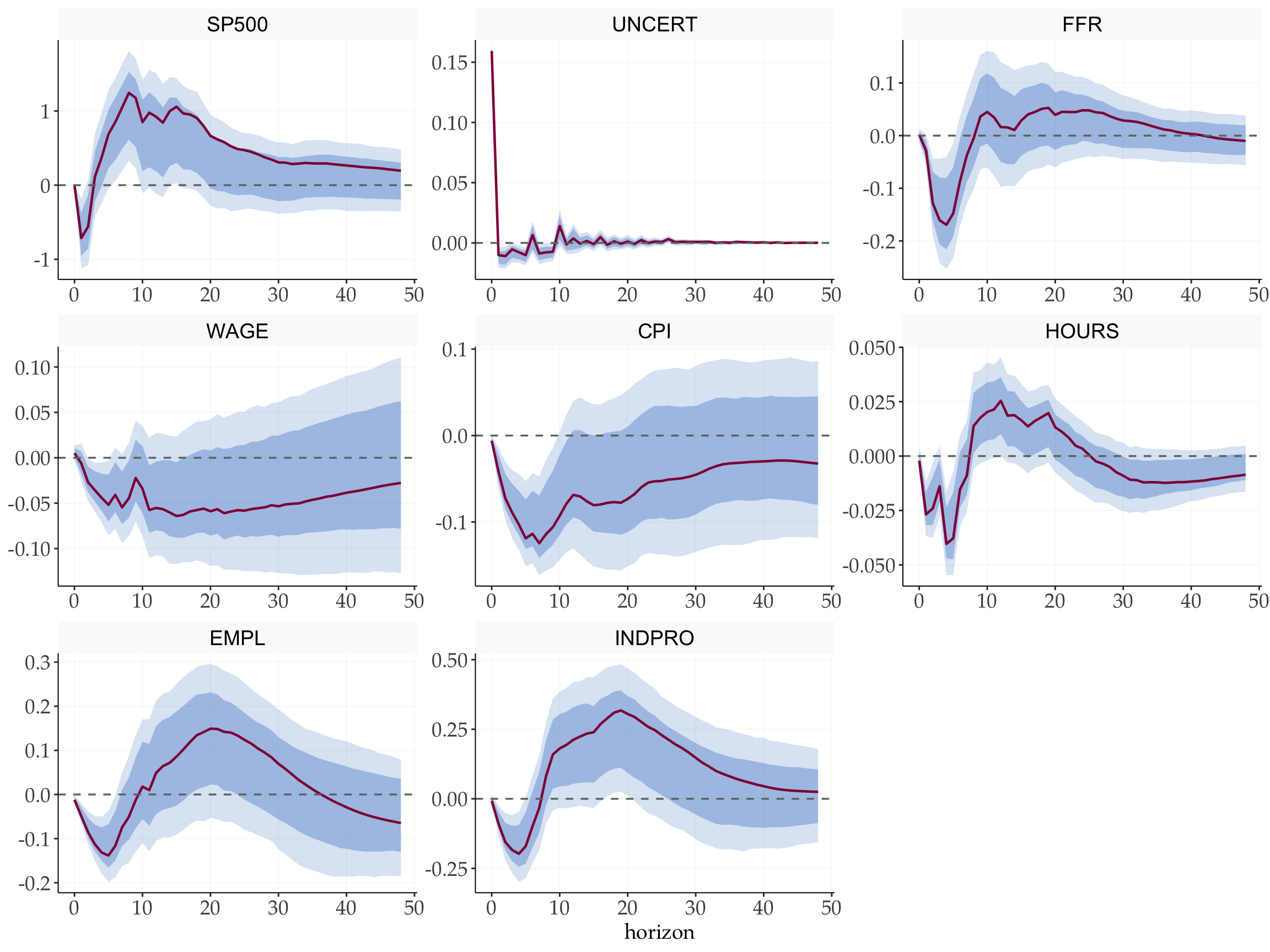

Figure 1: IRFs to uncertainty shock — standard bootstrap (68% and 90% confidence bands)

6.2 Bias-Corrected Bootstrap

fplotirf_chol(
    point       = point_irf,
    boot_result = bloom_corrected,
    shock       = shock,
    varnames    = var_names,
    facet_ncol  = 3
) + 
    labs(y = NULL)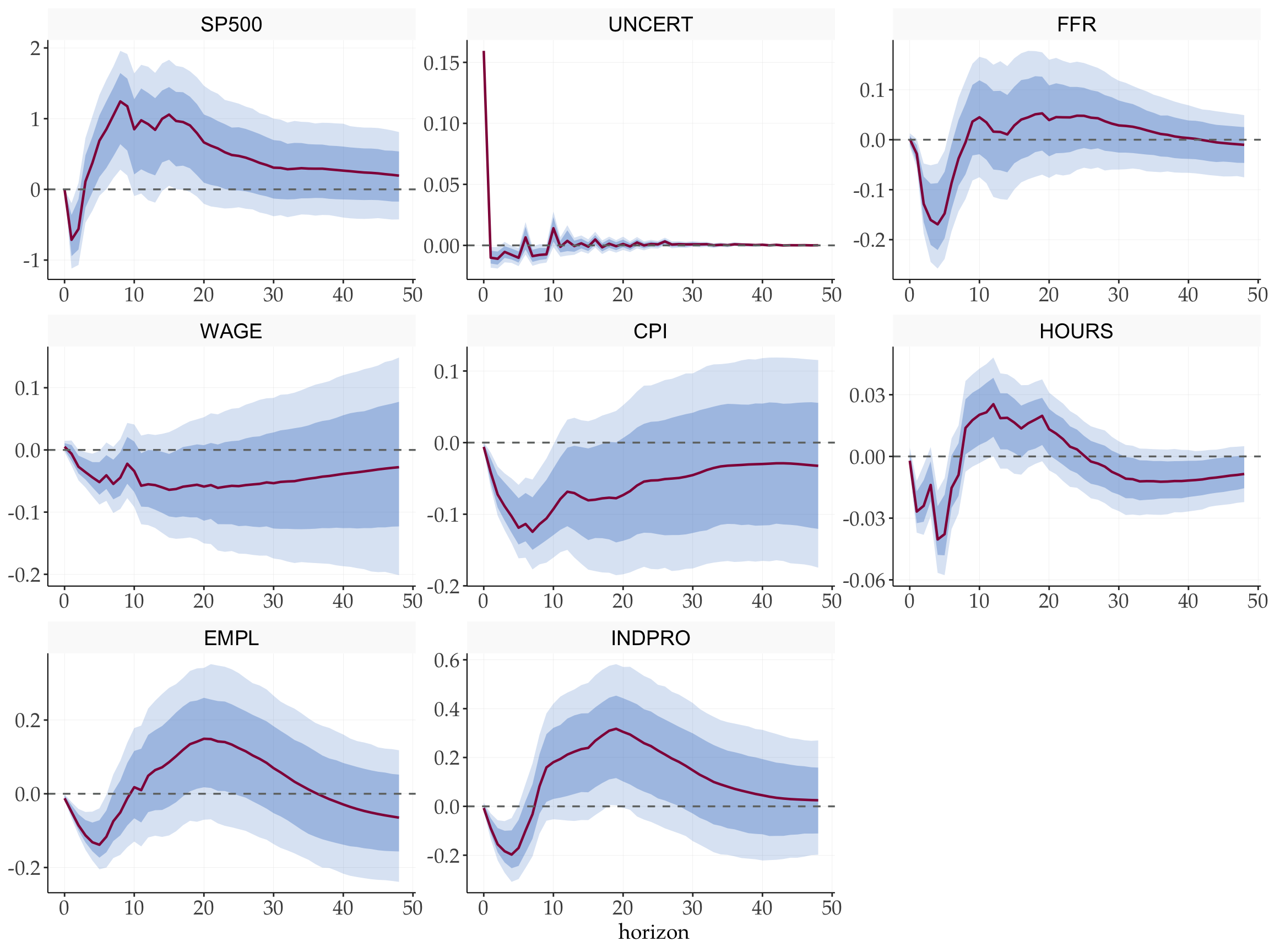

Figure 2: IRFs to uncertainty shock — bias-corrected bootstrap (68% and 90% confidence bands)

7 Forecast Error Variance Decomposition

vardec <- fevd_chol(point_irf, shock = shock)

fplot_vardec(
    fevd       = vardec$fevd,
    varnames   = var_names,
    shocknames = shockname
) +
  scale_fill_manual(values = tidyMacro_colors[c(2, 3)])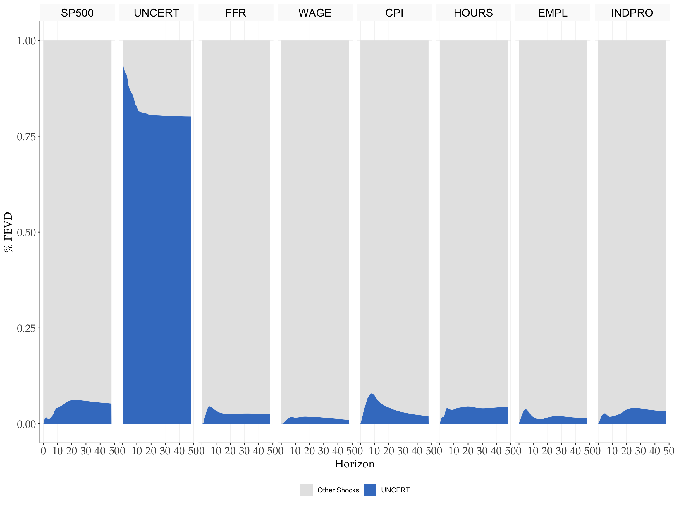

Figure 3: Forecast error variance decomposition: share explained by uncertainty shock

8 Historical Decomposition

# Exclude the shock variable itself from the response variables
series <- setdiff(seq_len(N), shock)

histdec_list <- setNames(
    lapply(series, function(i) fhistdec(y, var_bloom, S, i)$histdec),
    colnames(y)[series]
)

fplot_histdec(
    histdec_list = histdec_list,
    shock        = shock,
    shockname    = shockname,
    dates        = dates_vec,
    p            = p,
    facet_ncol   = 2
) +
    scale_x_date(date_breaks = "7 years", date_labels = "%Y")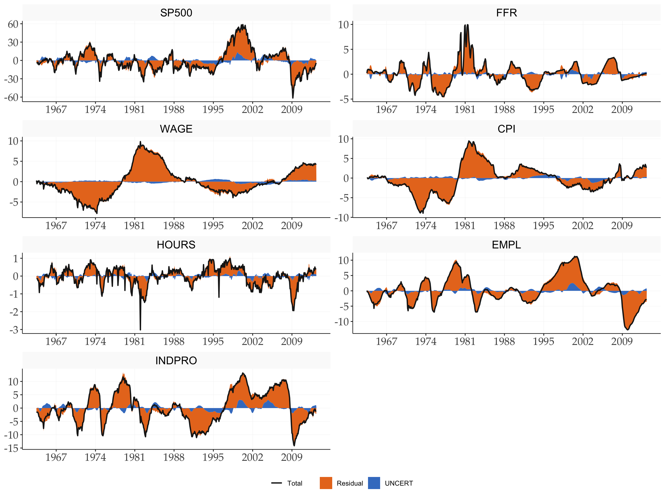

Figure 4: Historical decomposition: contribution of uncertainty shock

References

Bloom, Nicholas. 2009. “The Impact of Uncertainty Shocks.” Econometrica 77 (3): 623–85. https://doi.org/10.3982/ECTA6248.