library(tidyverse)
library(patchwork)
library(tidyMacro)Panel Local Projections
Micro Responses to Macro Shocks — Almuzara & Sancibrián (2024)
1 Overview
This chapter demonstrates fLPPanel() — tidyMacro’s panel local-projection estimator, a C++/OpenMP port of panel_LP.m from Almuzara and Sancibrián (2024). Shared conventions (formula grammar, ..macros, l()/f(), panel_id, output shapes, multi-band conf) are documented in the Local Projections syntax primer; this chapter focuses on the panel-specific estimator and replicates the reference R port on a synthetic unbalanced panel.
The estimated equation at horizon \(h\) (per \(j\)-th interaction component of \(s_{it}\,x_t\)) is \[y_{i,t+h} = \alpha^{(h)}_{\mathrm{FE}} + \beta_h^{(j)}\, (s_{it,j}\, x_t) + \gamma_h' w_{it} + \sum_{k=1}^{\min(h,\, p_{\max})} \delta_{hk}'\, v_{i,t-k} + u_{i,t+h}.\]
Estimator-specific arguments (beyond the shared list):
small_sample = TRUEinvokes the Imbens and Kolesár (2016) refinement, reporting a component-specific effective degrees of freedom instead of the default asymptotic \(t\)-clustered (LAHR) SE \(\hat V_h = (X'X)^{-1}\big(\sum_t Z_t Z_t'\big)(X'X)^{-1}\) with \(Z_t = \sum_i X_{it}\hat u_{it}\).p_maxcaps the number of lags of the regressand and the shock interaction added as controls (at horizon \(h\) the effective number is \(\min(h, p_\max)\)).cumulative = TRUEprojects \(\sum_{r=0}^{h} y_{i,t+r}\) instead of \(y_{i,t+h}\).
Output-side, fLPPanel() additionally exposes per-horizon status and converged vectors that flag no-complete-rows or HDFE non-convergence at individual horizons — the syntax primer’s output section explains the encoding.
2 Setup
3 A sample unbalanced panel
Note
The Almuzara and Sancibrián (2024) application uses proprietary firm-level Compustat/CRSP micro data. What follows is a synthetic sample panel built to have the same structure — a common macro shock, a cross-sectional characteristic that scales the response, unit and time fixed effects, and realistic missingness so that anyone can reproduce the workflow end-to-end.
set.seed(1918)

T_dim <- 30
N     <- 1000

# Common macro shock, unit-specific characteristic, true β = 1 on s·X.
macro <- rnorm(T_dim)
firm  <- 1 + rnorm(N)

df_bal <- data.frame(
  unit  = rep(1:N, times = T_dim),
  tt    = rep(1:T_dim, each  = N),
  shock = rep(macro, each  = N),
  size  = rep(firm,  times = T_dim)
) |>
  mutate(
    y = size * shock +
        as.vector(outer(0.5 * firm + rnorm(N), rnorm(T_dim))) +
        rnorm(n())
  )

# Realistic unbalancedness: (a) staggered entry, (b) random attrition,
# (c) sprinkled item-level NAs on the response.
set.seed(2025)
entry <- sample.int(6, N, replace = TRUE)          # entry at t ∈ 1..6
exit  <- pmin(T_dim, 14 + rgeom(N, prob = 0.15))   # exit at t ≥ 15
sparsity_mask <- runif(nrow(df_bal)) > 0.05        # drop 5% of surviving cells

df_panel <- df_bal |>
    dplyr::filter(tt >= entry[unit], tt <= exit[unit]) |>
    dplyr::filter(sparsity_mask[row_number()])
Coverage pattern for the first 60 firms:
df_panel |>
  filter(unit <= 60) |>
  ggplot(aes(x = tt, y = factor(unit))) +
    geom_point(size = 0.6, colour = "#0055A4") +
    scale_x_continuous(breaks = seq(0, T_dim, 5)) +
    labs(x = "t", y = "Firm id (first 60 firms)") +
    theme_minimal(base_size = 11) +
    theme(axis.text.y = element_blank())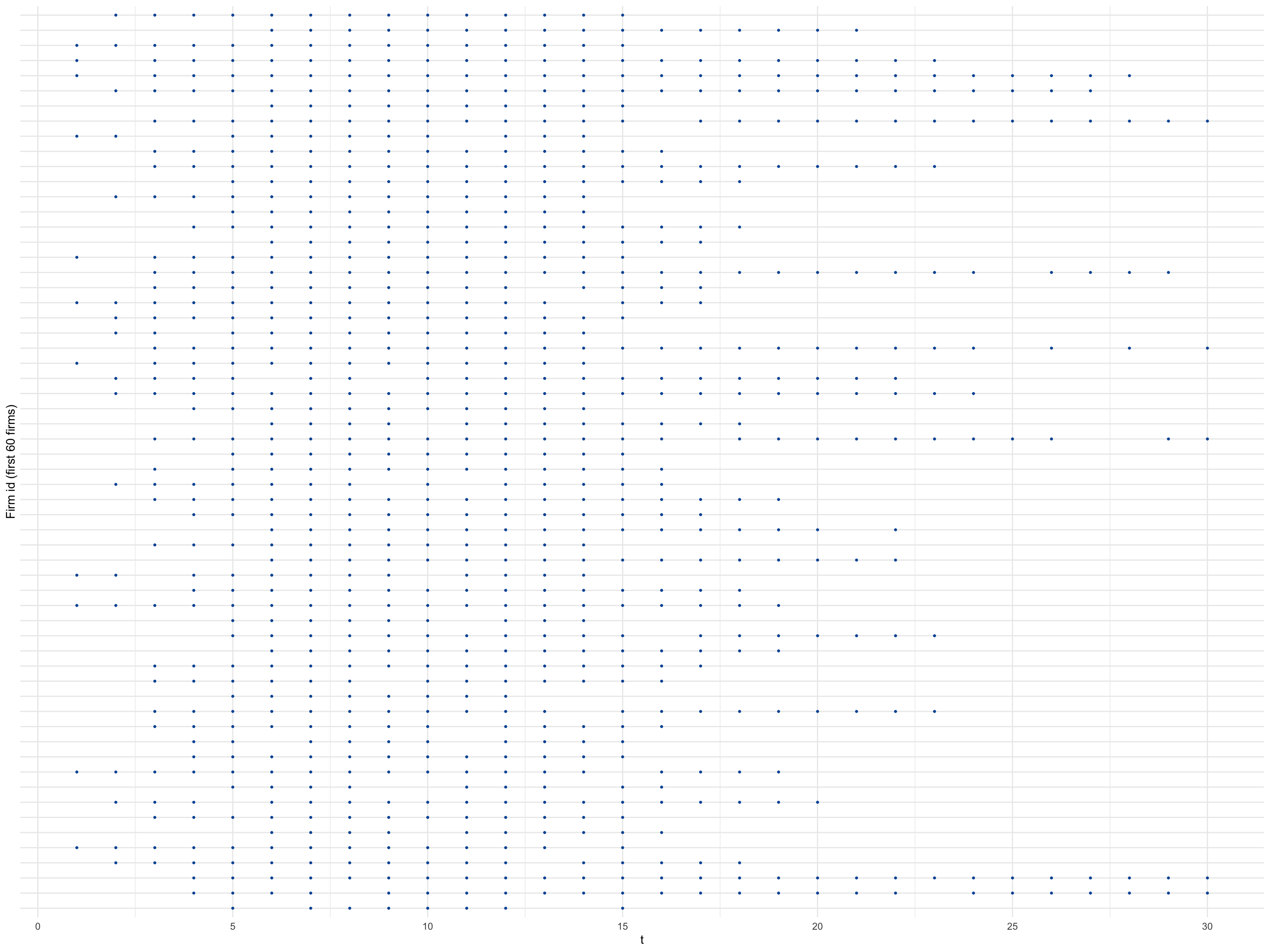
4 Estimation — one fLPPanel() call
The formula says exactly what the estimator does. shock:size is the elementwise product \(s_{it}\,X_t\) that generates cross-sectional variation (necessary once the unit-invariant shock is absorbed into tt fixed effects). Two-way FE go after |.
lp_pkg <- fLPPanel(
  y ~ shock:size | unit + tt,
  data         = df_panel,
  panel_id     = c("unit", "tt"),   # id + time in a single argument
  shock        = "shock:size",      # term label whose IRF we want
  horizons     = 5,
  conf         = c(68, 90),     # two bands from a single fit
  small_sample = TRUE,              # Imbens–Kolesar (2016) refinement
  cumulative   = TRUE,              # sum_{k=0..h} y_{i,t+k}
  n_threads    = 2                  # OpenMP over horizons
)
Tidy output:
tidyMacro:::tidy.fLPPanel(lp_pkg) |>
  mutate(across(where(is.numeric), \(x) round(x, 4)))
#>   horizon      shock estimate     se      df   pval lower_90 upper_90 lower_68
#> 1       0 shock:size   1.1025 0.0584 10.7029 0.0000   0.9973   1.2077   1.0416
#> 2       1 shock:size   1.3086 0.3235 10.7491 0.0020   0.7263   1.8908   0.9712
#> 3       2 shock:size   0.9401 0.4491 12.8419 0.0568   0.1440   1.7361   0.4755
#> 4       3 shock:size   0.4436 0.3659 11.8874 0.2489  -0.2090   1.0962   0.0639
#> 5       4 shock:size   0.7333 0.3406 11.3205 0.0537   0.1233   1.3433   0.3791
#> 6       5 shock:size   1.3550 0.3750 10.5620 0.0043   0.6789   2.0310   0.9636
#>   upper_68
#> 1   1.1634
#> 2   1.6459
#> 3   1.4046
#> 4   0.8233
#> 5   1.0875
#> 6   1.7463
5 Side-by-side check against fixest
fixest doesn’t ship a dedicated panel-LP function, but a cumulative panel LP is definitionally a stack of feols fits — one per horizon, with the leaded / cumulated regressand on the LHS and the same shock and fixed-effects on the RHS. We build that stack manually and compare it against fLPPanel() on the same unbalanced sample.
For an apples-to-apples comparison we fit fLPPanel() again with small_sample = FALSE so both estimators use asymptotic time-clustered (LAHR) standard errors.
library(fixest)

# Panel-aware cumulative-lead. IMPORTANT: `dplyr::lead(y, k)` shifts by
# ROW INDEX, so it silently closes internal time gaps in an unbalanced
# panel. To shift by actual TIME we first `complete()` the (unit, tt)
# grid — missing cells become NA — then `dplyr::lead` steps along real
# time, matching fLPPanel's per-unit hash-lookup shift.
df_grid <- df_panel |>
  tidyr::complete(unit, tt) |>
  dplyr::arrange(unit, tt)

lead_cumsum <- function(y, h) {
  s <- y                                              # h = 0 → y itself
  if (h > 0) for (k in 1:h) s <- s + dplyr::lead(y, k)
  s
}

H <- 5

fixest_tbl <- purrr::map_dfr(0:H, function(h) {
  df_h <- df_grid |>
    dplyr::group_by(unit) |>
    dplyr::mutate(y_h = lead_cumsum(y, h)) |>
    dplyr::ungroup() |>
    tidyr::drop_na(y_h, shock, size)      # drop grid cells that were empty

  fit <- fixest::feols(y_h ~ shock:size | unit + tt,
                       data    = df_h,
                       cluster = ~tt,      # time-clustered LAHR SE
                       notes   = FALSE)
  tibble::tibble(
    h        = h,
    estimate = coef(fit)[["shock:size"]],
    se       = fit$se[["shock:size"]]
  )
}) |>
  dplyr::mutate(
    lo90 = estimate - stats::qnorm(0.95) * se,
    hi90 = estimate + stats::qnorm(0.95) * se
  )
# Refit with asymptotic time-clustered SE for the fixest comparison.
lp_pkg_asy <- fLPPanel(
y ~ shock:size | unit + tt,
data = df_panel,
panel_id = c("unit", "tt"),
shock = "shock:size",
horizons = H,
conf = 90,
small_sample = FALSE, # asymptotic LAHR to match fixest
cumulative = TRUE,
n_threads = 2
)Point estimates coincide to machine precision — both fits solve the same OLS system on the same effective sample. Standard errors agree up to fixest’s finite-sample cluster multiplier \(G/(G-1)\cdot(N-1)/(N-k)\), which fLPPanel does not apply in its asymptotic LAHR mode:
cat(sprintf(
  "max |estimate diff| = %.3e\nmax |SE       diff| = %.3e  (fixest cluster small-sample multiplier)\n",
  max(abs(as.vector(lp_pkg_asy$irfs)    - fixest_tbl$estimate)),
  max(abs(as.vector(lp_pkg_asy$irfs_se) - fixest_tbl$se))
))
#> max |estimate diff| = 1.132e-14
#> max |SE       diff| = 2.882e-02  (fixest cluster small-sample multiplier)
horizons <- 0:H
blue <- "#0055A4"
mk_panel <- function(est, lo, hi, title) {
ggplot(data.frame(h = horizons, est = est, lo = lo, hi = hi), aes(x = h)) +
geom_hline(yintercept = 0, linetype = "dashed", linewidth = 0.4) +
geom_ribbon(aes(ymin = lo, ymax = hi), fill = blue, alpha = 0.2) +
geom_line(aes(y = est), colour = blue, linewidth = 1.2) +
geom_point(aes(y = est), colour = blue, size = 3) +
scale_x_continuous(breaks = horizons) +
labs(title = title, x = "h", y = "Cumulative response") +
theme_minimal(base_size = 13)
}
p_pkg <- mk_panel(as.vector(lp_pkg_asy$irfs),
as.vector(lp_pkg_asy$irfs_lower),
as.vector(lp_pkg_asy$irfs_upper),
"tidyMacro::fLPPanel()")
p_fx <- mk_panel(fixest_tbl$estimate,
fixest_tbl$lo90,
fixest_tbl$hi90,
"fixest::feols stack")
p_pkg + p_fx + plot_layout(ncol = 2)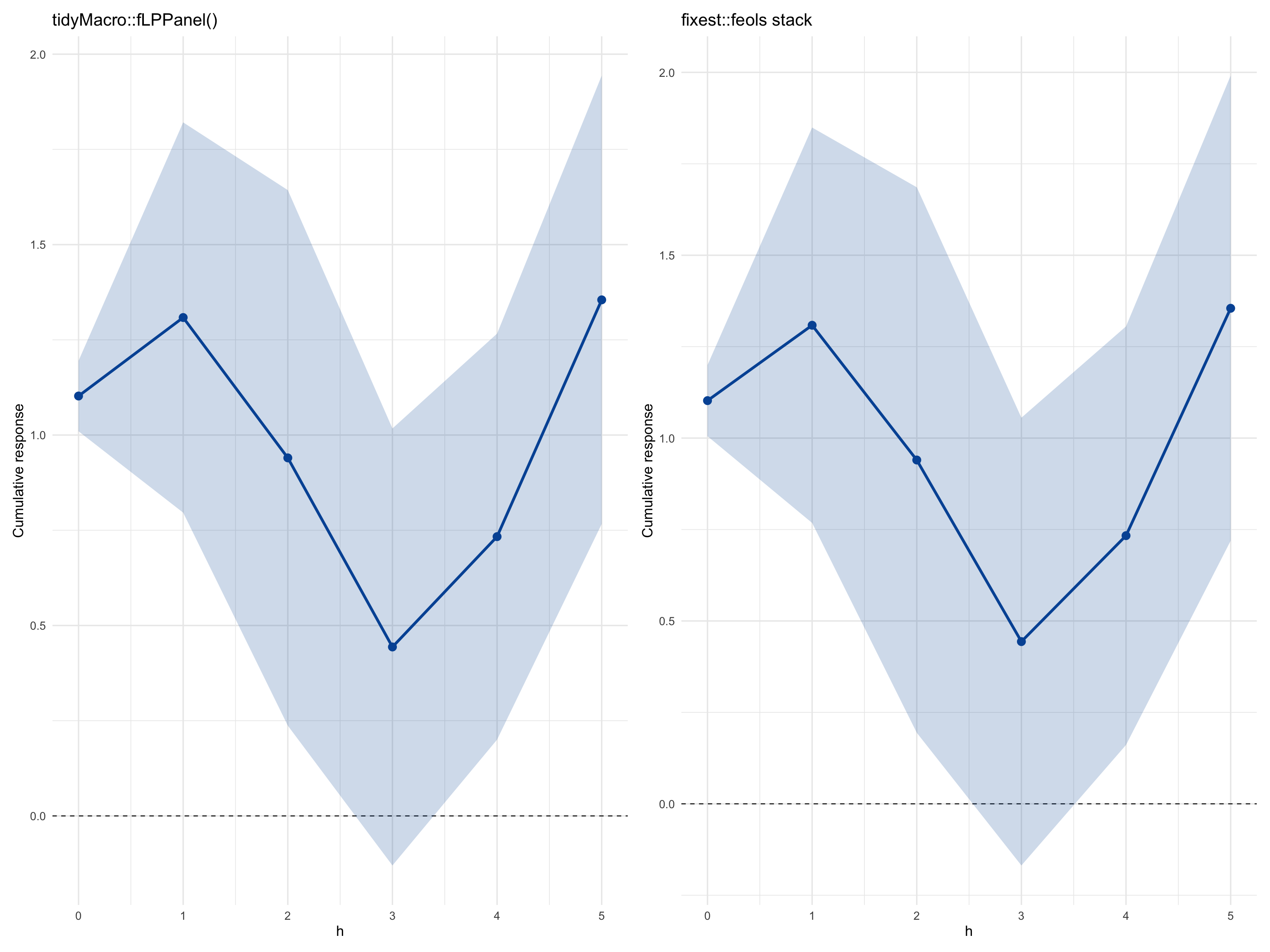
TipWhat
fLPPanel() adds over a raw fixest stack
- One call instead of one per horizon.
- Panel-aware
l()/f()operators that respect unit boundaries. - OpenMP-parallel horizon loop (each horizon is independent once y is leaded).
- Optional Imbens and Kolesár (2016) small-sample refinement with component-specific effective degrees of freedom (set
small_sample = TRUE; not infixest). - Multi-band CIs from a single fit (
conf = c(68, 95)).
6 Two-band plot via fPlotLP()
The result object has class c("fLPPanel", "fLP") so every fLP helper transfers:
fPlotLP(lp_pkg) +
  ggplot2::labs(x = "h", y = "Cumulative response")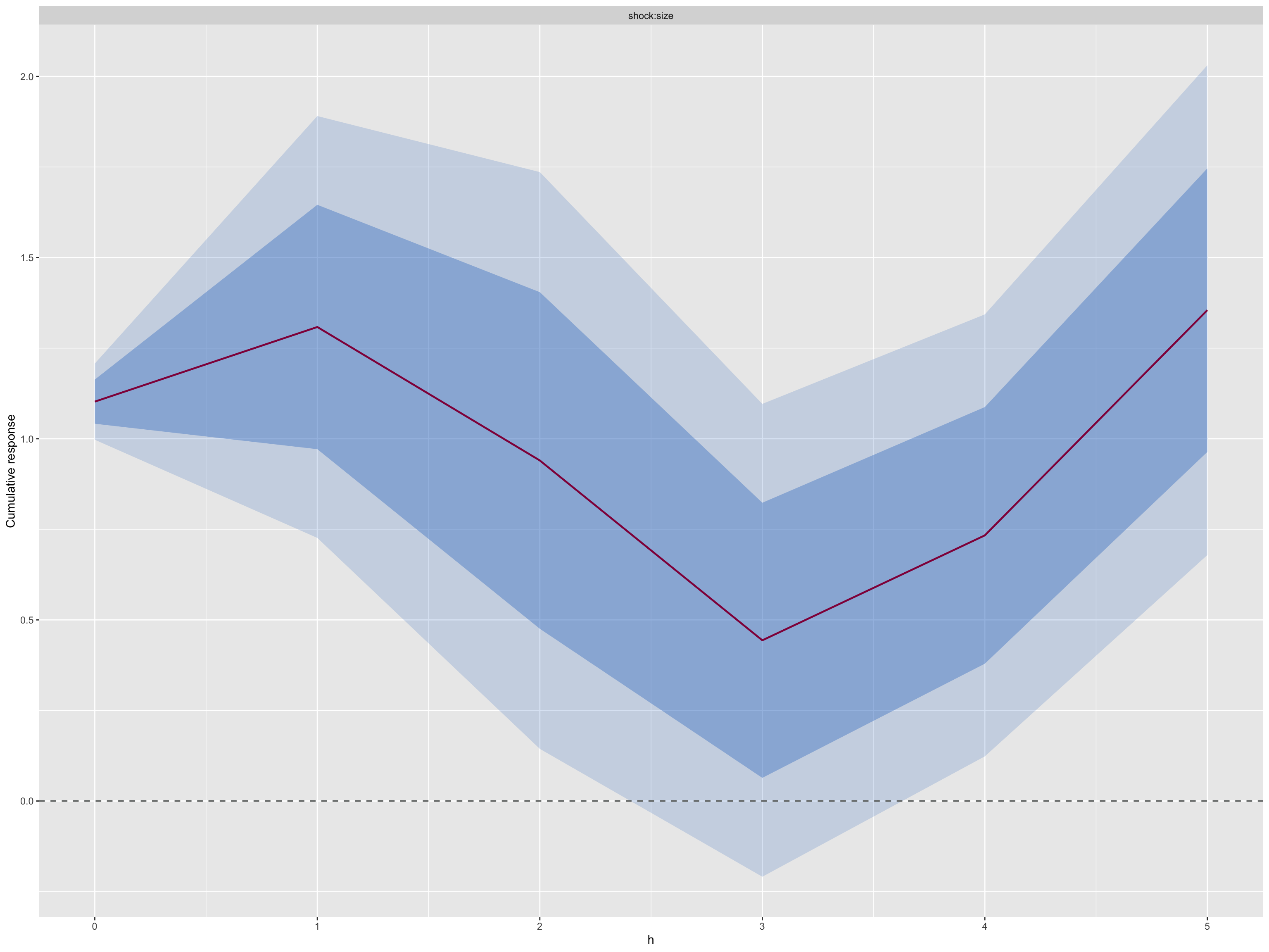
7 Other supported specifications
Alternative shapes — bare shock, no interaction, no fixed effects, panel-aware lags with macros — follow the shared formula grammar and are demonstrated in the Local Projections syntax primer. Everything documented there works with fLPPanel() unchanged.
References
Almuzara, Martı́n, and Vı́ctor Sancibrián. 2024. “Micro Responses to Macro Shocks.” FRB of New York Staff Report, no. 1090.
Imbens, Guido W., and Michal Kolesár. 2016. “Robust Standard Errors in Small Samples: Some Practical Advice.” The Review of Economics and Statistics 98 (4): 701–12. https://doi.org/10.1162/REST_a_00552.