library(tidyverse)
library(tidyMacro)
library(tictoc)

set_theme(fThemeTidyMacro())Long run restrictions
Technology, Employment, and the Business Cycle: Do Technology Shocks Explain Aggregate Fluctuations?
1 Overview
This document replicates the main empirical results of Galí (1999) shocks can have a permanent effect on labor productivity.
2 Model and Identification
With \(\Phi(1) = \sum_{h=0}^{\infty} \Phi_h\) the reduced-form long-run multiplier, the cumulative structural effect is \(\Theta(1) = \Phi(1) B_0\). The reduced form identifies the long-run covariance
\[\Omega \equiv \Phi(1)\, \Sigma\, \Phi(1)' = \Theta(1)\, \Theta(1)'.\]
Imposing a lower-triangular \(\Theta(1)\) (only technology shocks affect productivity permanently) makes it the unique Cholesky factor of \(\Omega\), and the impact matrix follows as
\[\Theta(1) = \operatorname{chol}(\Omega), \qquad B_0 = \Phi(1)^{-1}\, \Theta(1).\]
3 Setup
4 Data
data("Gali1999")
Gali1999 |> head()
#> # A tibble: 6 × 3
#>   Date       Productivity  Hours
#>   <date>            <dbl>  <dbl>
#> 1 1947-04-01         2.01 -0.507
#> 2 1947-07-01        -3.20  3.09
#> 3 1947-10-01         3.82  3.03
#> 4 1948-01-01        12.0  -1.99
#> 5 1948-04-01         9.54  0.186
#> 6 1948-07-01        -3.11  3.63
y <- Gali1999 |> select(Productivity, Hours) |> as.matrix()
dates <- Gali1999 |> pull(Date)
T <- nrow(y)
N <- ncol(y)5 VAR Estimation
# Lag length selection via AIC
p <- fAICBIC(y, pmax = 4, c = 1)$aic
c <- 1

# Estimate VAR
var_result <- fVAR(y, p = p, c = c)

# Variance-covariance matrix of reduced-form residuals
Sigma <- var_result$sigma
6 BQ Identification
horizon <- 40
wold <- fWoldIRF(var_result, horizon = horizon)

# Long-run multiplier matrix
C1 <- apply(wold, c(1, 2), sum)

# Lower Cholesky of long-run covariance
D1 <- t(chol(C1 %*% Sigma %*% t(C1)))

# Structural impact matrix
K <- solve(C1, D1)

# BQ IRFs (in first differences)
irf_bq <- fBQIRF(wold, K)
7 Bootstrap Confidence Bands
tic()
boot_bq <- fBootstrapBQ(
  y = y,
  var_result = var_result,
  nboot = 1000,
  horizon = 40,
  bootscheme = "residual",
  cumulate = c(1, 2)
)
toc()
#> 0.058 sec elapsed
8 Impulse Response Functions
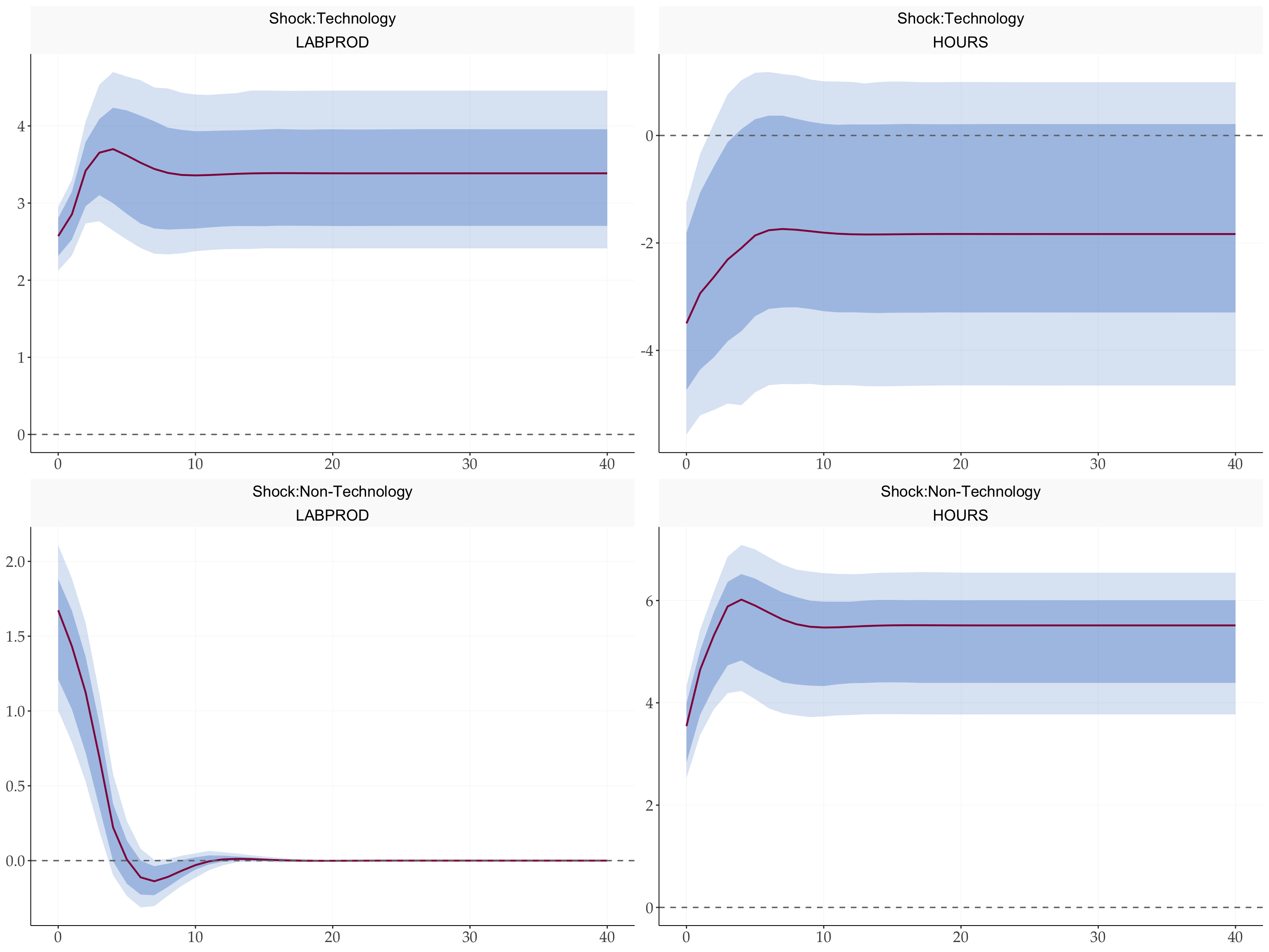
Level responses are recovered by accumulating the first-differenced IRFs. The first shock is the technology shock; the second is the non-technology shock.
fPlotIRFBQ(
  point       = irf_bq,
  boot_result = boot_bq,
  varnames    = c("LABPROD", "HOURS"),
  shocknames  = c("Shock:Technology", "Shock:Non-Technology"),
  cumulate    = c(1, 2),
  shocks      = c(1, 2)
)
9 Forecast Error Variance Decomposition
# Cumulate BQ IRF along horizon (dim 3) to get level responses
irf_cumu <- irf_bq
for (h in 2:dim(irf_bq)[3]) {
  irf_cumu[, , h] <- irf_cumu[, , h] + irf_cumu[, , h - 1]
}

# FEVD — reuses Cholesky FEVD function (same maths)
fevd <- fFEVDChol(irf_cumu, shock = 0)$fevd
fevd <- fevd[, c(2, 1), ] # optional, for vis purposes

fPlotVarDec(
  fevd = fevd,
  varnames = c("LABPROD", "HOURS"),
  shocknames = c("Technology", "Non-Technology")
) +
  scale_fill_manual(values = tidyMacro_colors[1:2])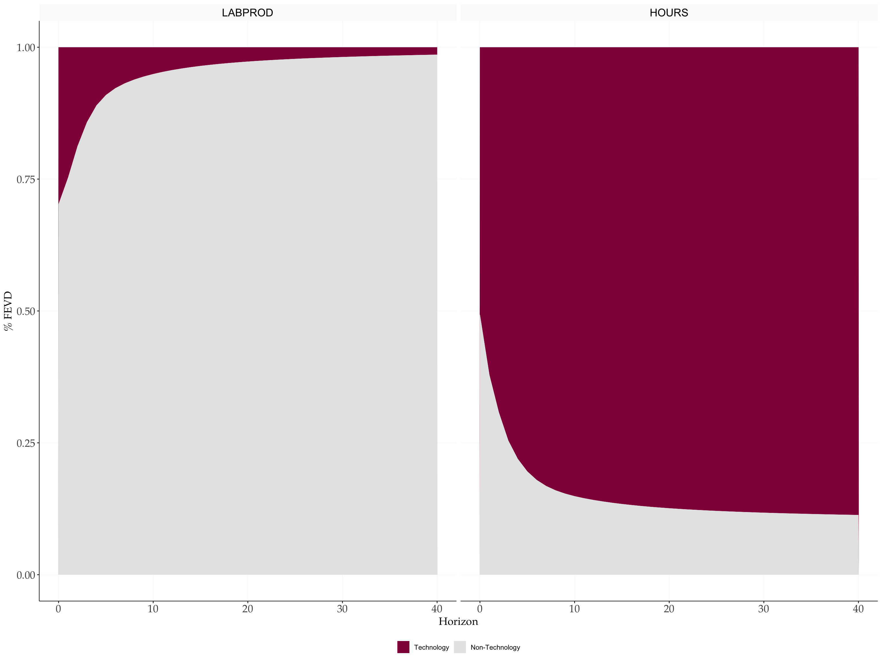
10 Historical Decomposition
histdec_all <- vector("list", N)
ystar_all <- matrix(0, nrow = T - p, ncol = N)

for (series in seq_len(N)) {
  res <- fHistDec(y, var_result, K, series)
  histdec_all[[series]] <- res$histdec
  ystar_all[, series] <- res$ystar
}

names(histdec_all) <- c("LABPROD", "HOURS")

fPlotHistDec(
  histdec_list = histdec_all,
  shock = 1,
  shockname = "Technology",
  dates = dates,
  p = p,
  facet_ncol = 1
) +
  scale_x_date(date_breaks = "6 years", date_labels = "%Y")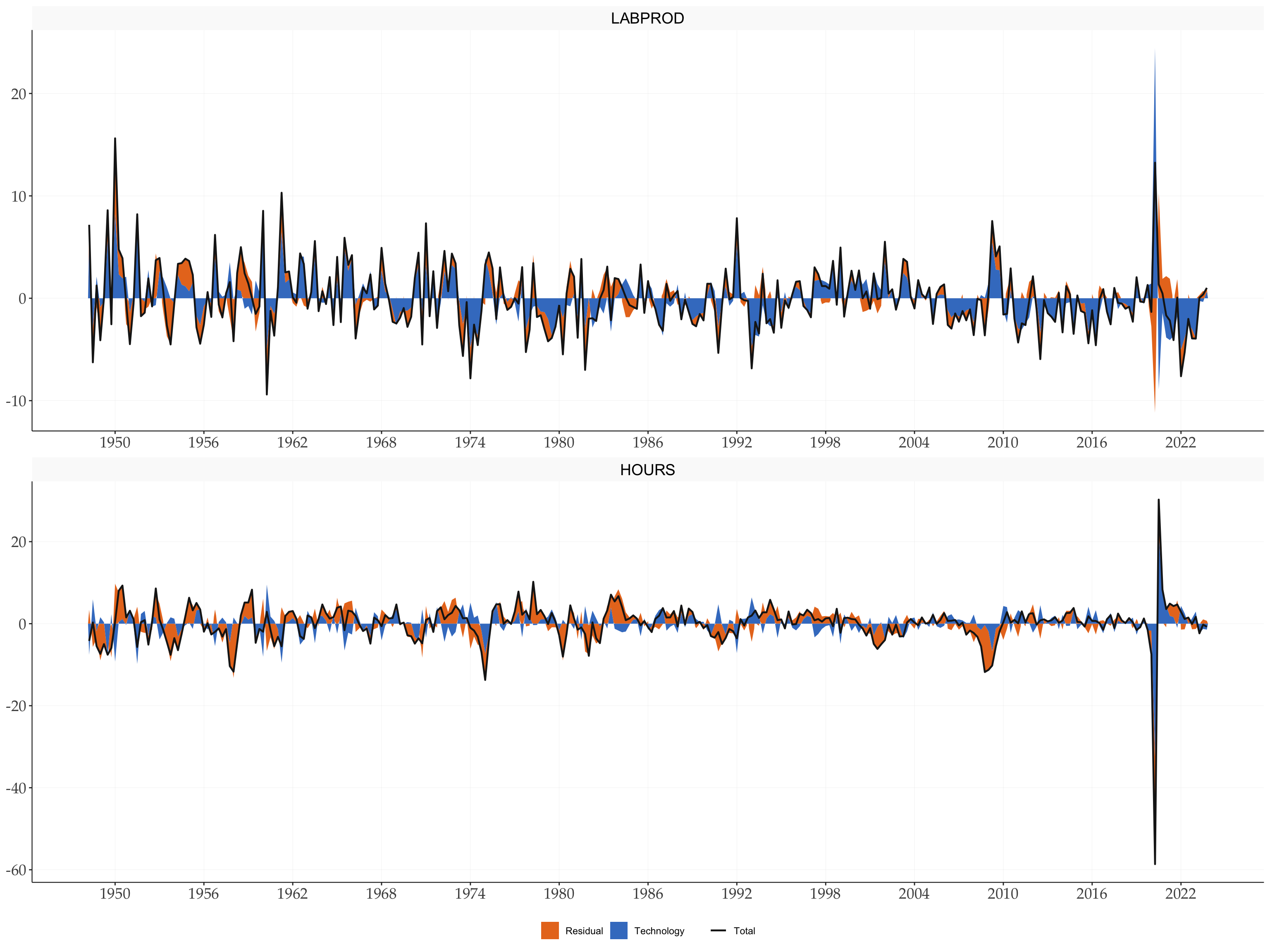
11 Conditional Correlations
Following Galí (1999) , we decompose the unconditional correlation between hours and productivity into shock-specific conditional correlations. The conditional correlation for shock \(i\) is:
\[\rho_i = \frac{\sum_{h} \theta_{1i,h}\, \theta_{2i,h}} {\sqrt{\left(\sum_{h} \theta_{1i,h}^2\right) \left(\sum_{h} \theta_{2i,h}^2\right)}},\]
where \(\theta_{ki,h}\) is the response of variable \(k\) to shock \(i\) at horizon \(h\).
# Dimensions of irf_bq: [variables, shocks, horizon]
N_shocks <- dim(irf_bq)[2]

# Numerator: for each shock i, sum of cross-products of IRFs of var 1 and var 2
numerator <- numeric(N_shocks)
for (i in 1:N_shocks) {
  temp         <- irf_bq[1, i, ] * irf_bq[2, i, ]
  numerator[i] <- sum(temp)
}

# Denominator: sqrt of product of sum-of-squares for each shock
irf_squared <- irf_bq^2
denominator <- numeric(N_shocks)
for (i in 1:N_shocks) {
  v1             <- sum(irf_squared[1, i, ])
  v2             <- sum(irf_squared[2, i, ])
  denominator[i] <- sqrt(v1 * v2)
}

# Conditional correlations (one per shock)
cond_corr <- numerator / denominator

# Unconditional correlations
uncond_corr <- cor(y)

cat("Unconditional correlation (Productivity, Hours):", round(uncond_corr[1, 2], 3), "\n")
#> Unconditional correlation (Productivity, Hours): -0.203
cat("Conditional correlation | Technology shock:     ", round(cond_corr[1], 3), "\n")
#> Conditional correlation | Technology shock:      -0.901
cat("Conditional correlation | Non-Technology shock: ", round(cond_corr[2], 3), "\n")
#> Conditional correlation | Non-Technology shock:  0.733
Hours and productivity are nearly uncorrelated unconditionally, which sits uncomfortably with standard RBC theory. Once we condition on the source of variation, the picture sharpens: technology improvements are accompanied by a decline in hours, producing a negative conditional correlation. It is the non-technology shock that drives hours and productivity in the same direction — precisely the co-movement that RBC models mistakenly ascribed to technology.
References
Galí, Jordi. 1999. “Technology, Employment, and the Business Cycle: Do Technology Shocks Explain Aggregate Fluctuations?” American Economic Review 89 (1): 249–71. https://doi.org/10.1257/aer.89.1.249.