10  Local Projections with Shocks and IV

A guided tour via Jordà and Taylor (2025)

10.1 Overview

This chapter is a replication of Jorda and Taylor (2025) with fLP() and fLPIV(). Syntax conventions common to all four local-projection engines — formulas, ..macros, l()/f(), multi-band conf, thread rules, output shapes — live in the Local Projections syntax primer; this chapter focuses on the empirical exercise.

The empirical exercise projects log CPI (×100) on a unit Romer-Romer monetary policy shock over 1985Q1-2007Q4, using long differences CPI_{t+h} - CPI_{t-1} and four lags of real GDP growth, CPI inflation, and the short-term rate change as controls. Two features specific to reproducing Jorda and Taylor (2025) in MATLAB (LPmodel.m) matter here:

• The Newey-West bandwidth rule is Jordà’s classic = h, i.e. nw_offset = 0 (the syntax primer explains the default). Under this rule the standard errors match OLSmodel.m bit-for-bit.
• The LP-IV specification uses a fixed HAC bandwidth of 6 (nw_lags_iv = 6), matching Stata’s vce(hac nw 6).

---

10.2 Setup

library(tidyverse)
library(tidyMacro)
library(zoo)
library(patchwork)

set_theme(fThemeTidyMacro())

---

10.3 Data

data("JordaTaylor2025")

jt_lp <- JordaTaylor2025 |>
  mutate(Date = as.Date(as.yearqtr(Date, format = "%YQ%q"))) |>
  dplyr::filter(Date >= "1984-10-01", Date <= "2007-10-01") |>
  transmute(
      Date,
      CPI = 100 * logCPI,
      RRShock,
      dLogGDP,
      dLogCPI,
      dSTIR
    )

jt_lp |> head()
#> # A tibble: 6 × 6
#>   Date         CPI RRShock dLogGDP dLogCPI   dSTIR
#>   <date>     <dbl>   <dbl>   <dbl>   <dbl>   <dbl>
#> 1 1984-10-01 -57.8 -0.742     3.76    2.68 -2.12  
#> 2 1985-01-01 -56.7  0.0864    4.16    4.57 -0.790 
#> 3 1985-04-01 -56.1 -0.146     3.48    2.47 -0.560 
#> 4 1985-07-01 -55.5  0.251     6.14    2.31 -0.0200
#> 5 1985-10-01 -54.9  0.0732    2.48    2.31  0.200 
#> 6 1986-01-01 -54.4 -0.0949    4.09    1.95 -0.270

jt_lp |>
  slice(-1) |>
  select(Date, CPI, RRShock, dLogGDP, dSTIR) |>
  pivot_longer(-Date, names_to = "variable") |>
  ggplot(aes(x = Date, y = value)) +
    geom_line(linewidth = 0.7) +
    facet_wrap(~ variable, scales = "free", ncol = 2) +
    scale_x_date(date_labels = "%Y.%m") +
    labs(x = NULL, y = NULL)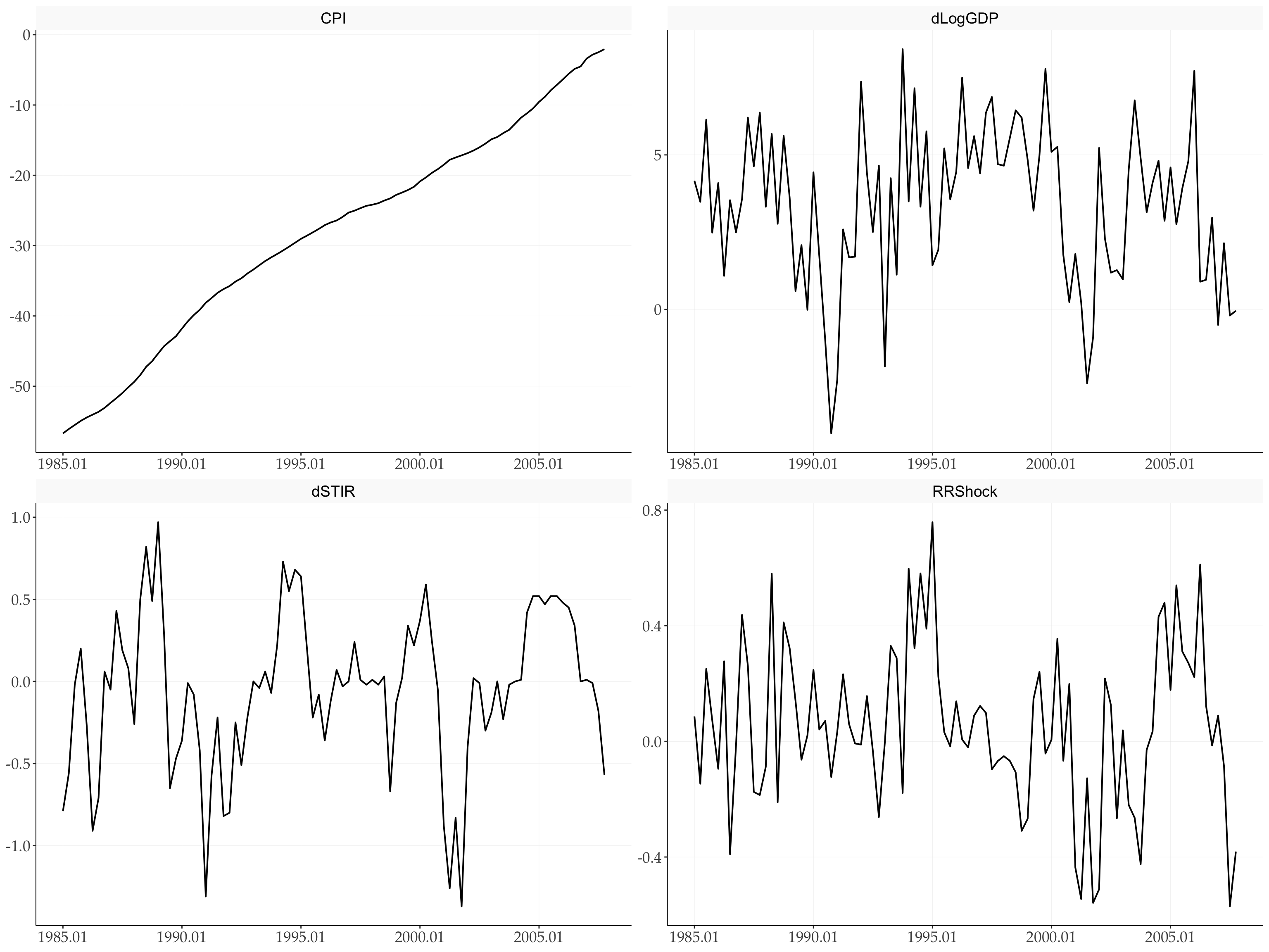

Figure 10.1: Variables used in the LP replications

---

10.4 1 · Classic LP-OLS replication — one fit, two bands

The Jordà-Taylor (2025) result. A single call to fLP() delivers both the 68% and 95% bands: pass conf = c(0.68, 0.95) and the bands are rebuilt from the raw irfs_se in the fit object — no need to estimate twice.

controls <- c("dLogGDP", "dLogCPI", "dSTIR")

lp_jt <- fLP(
  CPI ~ RRShock + l(..controls, 1:4),
  data       = jt_lp,
  horizons   = 18,
  shock      = "RRShock",
  conf       = c(0.68, 0.95),   # multi-band from one fit
  nw_lags    = 0,
  nw_offset  = 0,               # classic Jordà rule; matches OLSmodel.m
  cumulative = TRUE,
  n_threads  = 1
)

10.4.1 Direct plot

fPlotLP() draws one ribbon per band automatically (widest first, so the tighter band sits visually on top).

p1 <- fPlotLP(lp_jt) +
  labs(title = "CPI response to a unit Romer-Romer shock (Auto)",
       y = "Percent")

10.4.2 Customized plot from tidy data

Every plot can also be assembled by hand from the tidy plot data.

p2 <- fPlotLP(lp_jt, return_data = TRUE) |>
  ggplot(aes(x = horizon, y = point)) +
    geom_ribbon(aes(ymin = lower, ymax = upper, group = conf, alpha = conf, fill = NULL),
                fill = "#407EC9") +
    geom_line(linewidth = 0.9, colour = "#910048") +
    geom_hline(yintercept = 0, linewidth = 0.4, linetype = "dashed") +
    scale_alpha_manual(values = c(`0.95` = 0.18, `0.68` = 0.34)) +
    scale_x_continuous(breaks = seq(0, 15, 5)) +
    labs(title = "CPI response to Romer-Romer shock (Manual)", y = "Percent")


# Compare charts
p1 + p2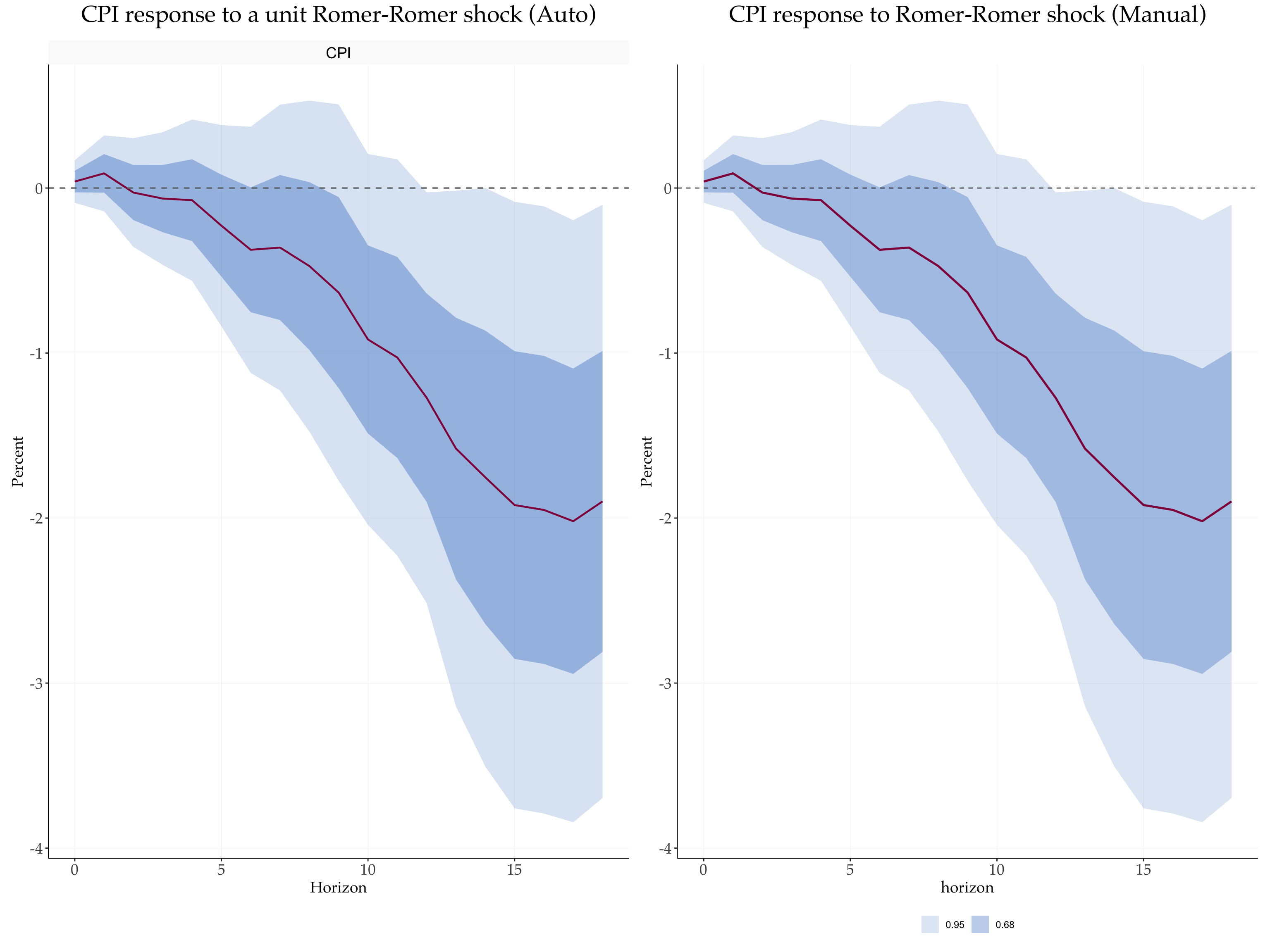

Figure 10.2: Same fit, hand-rolled ggplot from fPlotLP(..., return_data = TRUE)

---

10.5 2 · Many responses to one shock: Multi-equation LHS

fLP() accepts a vector-valued LHS: c(y1, y2, y3) ~ shock + .... Each LHS variable is estimated as its own local projection against the shared RHS — in parallel across horizons (OpenMP) — and returned as a single fLP object. Combined with conf = c(0.68, 0.95), one call yields a full multi-response × multi-band figure.

lp_multi <- fLP(
  c(CPI, dSTIR) ~ RRShock + l(..controls, 1:4),
  data       = jt_lp,
  horizons   = 17,
  shock      = "RRShock",
  conf       = c(0.68, 0.95),
  nw_lags    = 0,
  nw_offset  = 0,
  cumulative = TRUE,
  n_threads  = 1
)

fPlotLP(lp_multi, facet_ncol = 2) +
  labs(title = "Responses to a Romer-Romer shock (1 fit, 2 LHS × 2 bands)")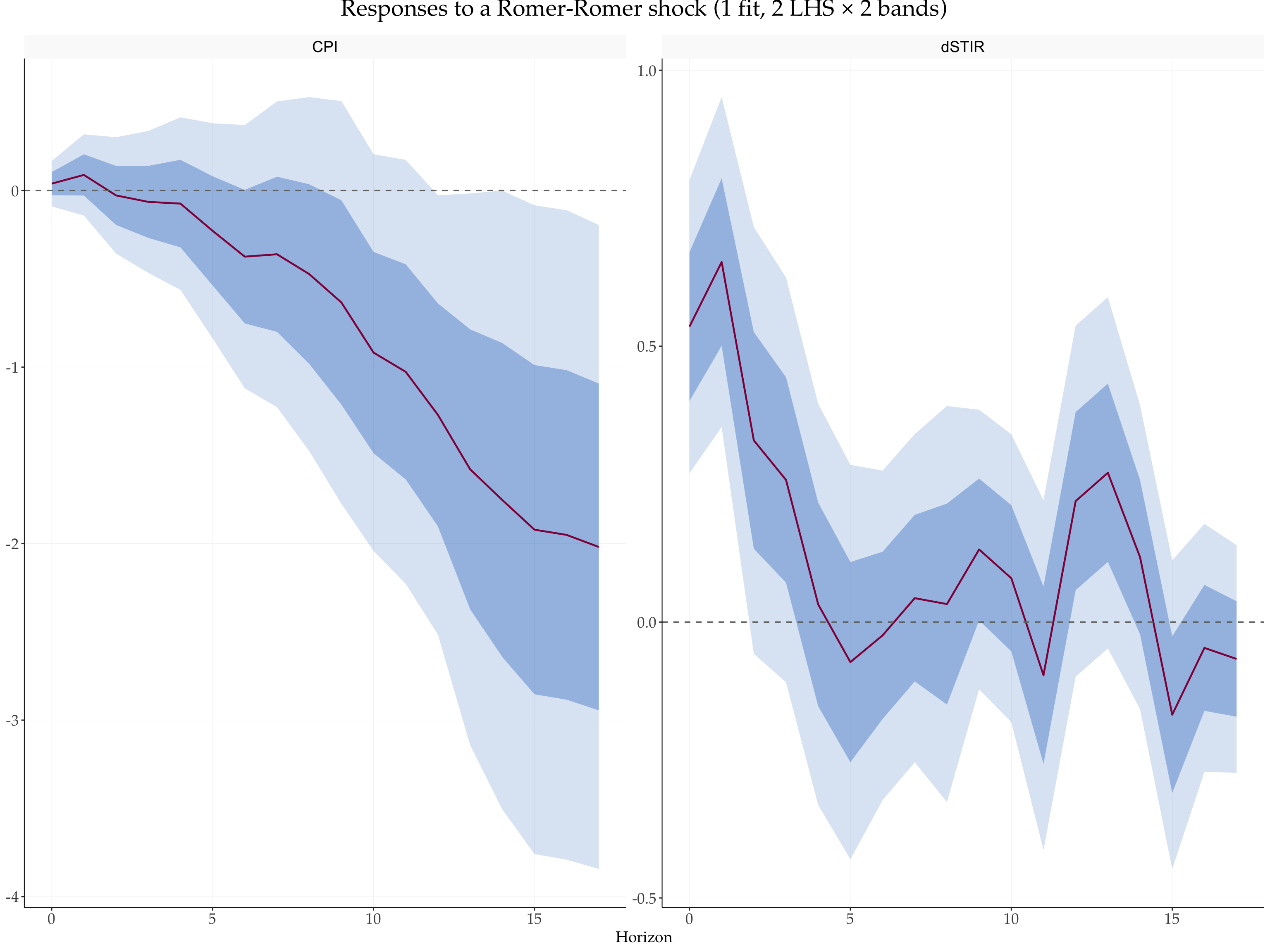

Figure 10.3: Multi-equation LP — two responses to one Romer-Romer shock, one fit

Behind the scenes each response has its own regression; only the RHS is shared. This is materially faster than looping in R because the horizon loop is parallelised in C++ and only the OLS cross-products are formed once per horizon. Note also that fLP() does not auto-augment the RHS — the RHS you write is exactly what enters each regression. For instance, above the dSTIR equation happens to have dSTIR_l1..l4 on the RHS only because dSTIR is a member of the ..controls macro; if you drop it from controls, its own lags disappear from the RHS.

---

10.6 3 · Level vs cumulative responses

cumulative = TRUE regresses y_{t+h} - y_{t-1} on the RHS; FALSE regresses the level y_{t+h}. Comparing them makes the “level” vs “long-difference” distinction explicit.

lp_cum <- fLP(
    CPI ~ RRShock + l(..controls, 1:4),
    data = jt_lp, 
    horizons = 17, 
    shock = "RRShock",
    conf = c(0.68, 0.90), 
    nw_lags = 0, 
    nw_offset = 0,
    cumulative = TRUE,  
    n_threads = 1
)

lp_lev <- fLP(
    CPI ~ RRShock + l(..controls, 1:4),
    data = jt_lp, 
    horizons = 17, 
    shock = "RRShock",
    conf = c(0.68, 0.90), 
    nw_lags = 0, 
    nw_offset = 0,
    cumulative = FALSE,  
    n_threads = 1
)

fPlotLP(lp_cum) + ggtitle('Cumulative Response') + fPlotLP(lp_lev) + ggtitle('Level Response')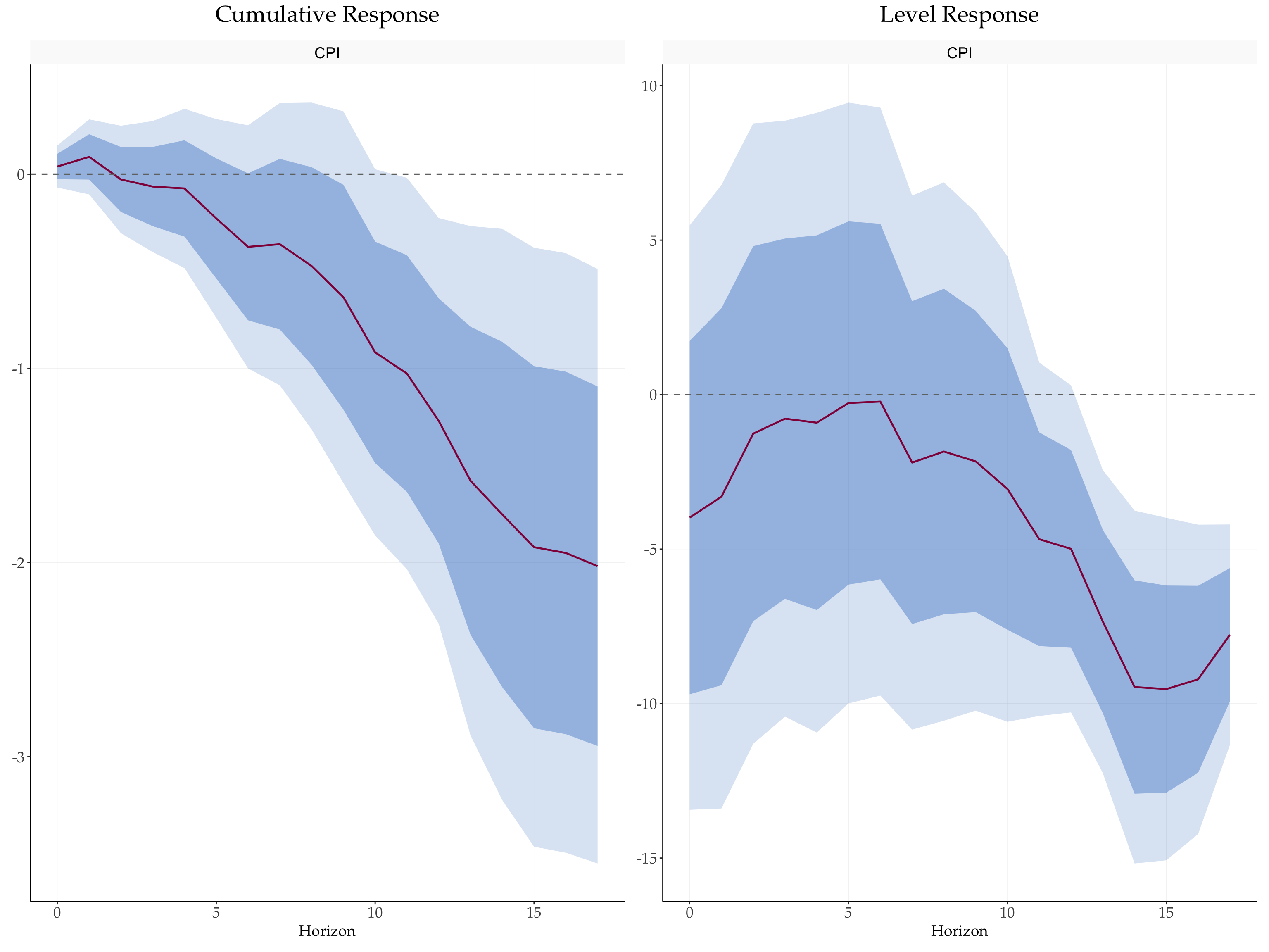

---

10.7 4 · Newey-West bandwidth: matching MATLAB vs the MA&R default

Two bandwidth rules give identical point estimates but different SE bands: the classic Jordà = h rule (nw_offset = 0, matches LPmodel.m bit-for-bit) and the Miranda-Agrippino & Ricco = h + 1 rule (nw_offset = 1, the fLP() default). The syntax primer covers the general convention; here we visualise the resulting band gap on this replication.

lp_jorda <- fLP(CPI ~ RRShock + l(..controls, 1:4),
                data = jt_lp, horizons = 17, shock = "RRShock",
                conf = 0.90, nw_lags = 0, nw_offset = 0,
                cumulative = TRUE, n_threads = 1)

lp_mar   <- fLP(CPI ~ RRShock + l(..controls, 1:4),
                data = jt_lp, horizons = 17, shock = "RRShock",
                conf = 0.90, nw_lags = 0, nw_offset = 1,
                cumulative = TRUE, n_threads = 1)

# IRFs are identical; only the NW bandwidth (and hence SEs) differ.
all.equal(as.numeric(lp_jorda$irfs), as.numeric(lp_mar$irfs))
#> [1] TRUE

bind_rows(
  fPlotLP(lp_jorda, return_data = TRUE) |> mutate(rule = "Jordà (h)"),
  fPlotLP(lp_mar,   return_data = TRUE) |> mutate(rule = "Miranda-Agrippino (h+1)")
) |>
  ggplot(aes(x = horizon, y = point, colour = rule, fill = rule)) +
    geom_ribbon(aes(ymin = lower, ymax = upper, color = rule), alpha = 0.5) +
    geom_line(linewidth = 0.9) +
    geom_hline(yintercept = 0, linewidth = 0.4, linetype = "dashed") +
    labs(title = "CPI response — NW bandwidth comparison at 90%",
         x = "Horizon", y = "Percent", colour = NULL, fill = NULL)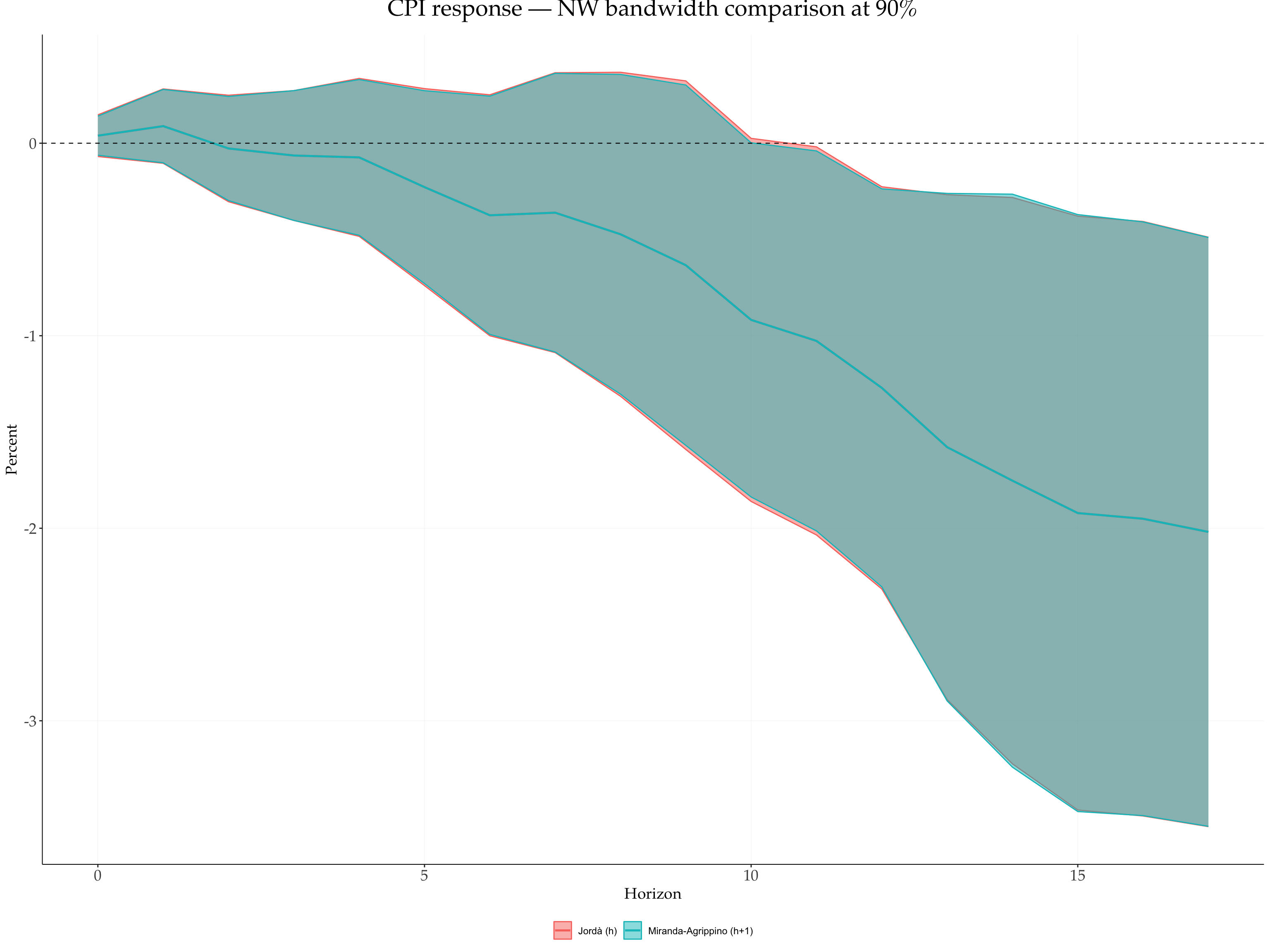

Figure 10.4: Same IRF, different NW bandwidth rule at 90%

---

10.8 5 · LP-IV — Unemployment response to an FFR shock

fLPIV() estimates local projections with an external instrument, mirroring fLP()’s formula-based syntax. Replicates Jordà & Taylor (2025) Figure 6a: the unemployment response to a unit federal-funds-rate shock, instrumented by the Romer-Romer (RR) narrative shock.

The specification (Ex6 tab of the JT2025 workbook, monthly 1985M1-2000M1):

• LHS: Unemployment (long difference, y_{t+h} - y_{t-1})
• Endogenous treatment: FFRates (the fed funds rate)
• Exogenous controls: six lags of Unemployment, Inflation, FFRates
• Instruments: contemporaneous RR shock plus six lags (over-identified 2SLS)
• HAC: Newey-West with a fixed bandwidth of 6 (Stata’s vce(hac nw 6))

The result is delivered horizon-by-horizon via Frisch-Waugh-Lovell 2SLS with a delta-method HAC standard error — the same recipe as Cesa-Bianchi’s LPmodel.m in LP-IV mode.

data("JordaTaylor2025IV")

jt_iv <- JordaTaylor2025IV |>
  filter(Date >= as.POSIXct("1985-01-01"),
         Date <= as.POSIXct("2000-01-01")) |>
  transmute(Date,
            urate = Unemployment,
            infl  = Inflation,
            ffr   = FFRates,
            rz    = RRShock)

jt_iv |>
  pivot_longer(-Date, names_to = "variable") |>
  ggplot(aes(x = Date, y = value)) +
    geom_line(linewidth = 0.7) +
    facet_wrap(~ variable, scales = "free", ncol = 2) +
    labs(x = NULL, y = NULL)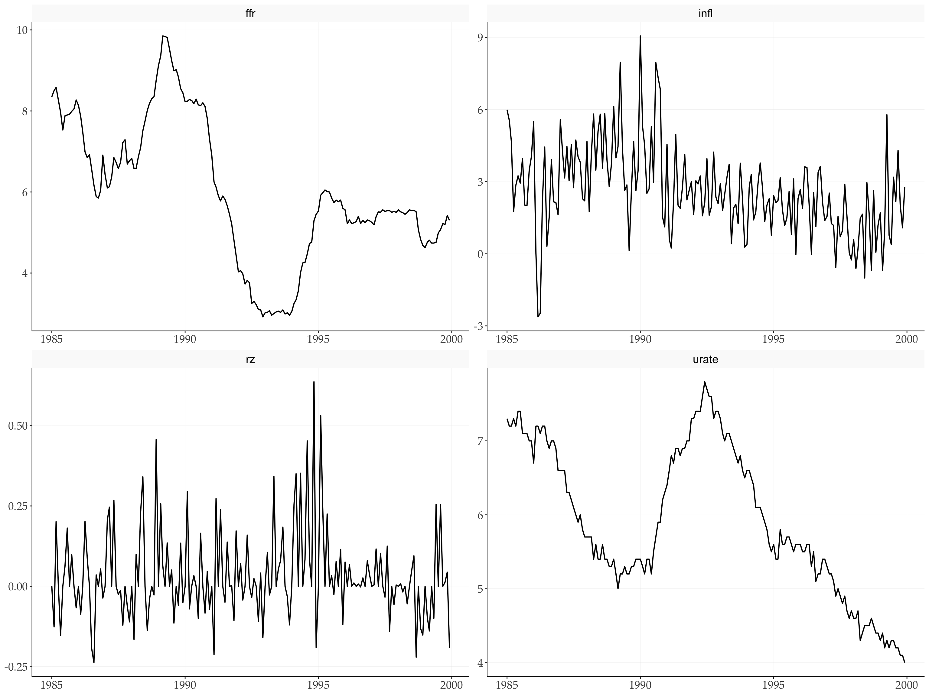

Figure 10.5: Variables used in the LP-IV replication

iv_ctrl <- c("urate", "infl", "ffr")

lp_iv <- fLPIV(
  urate ~ ffr + l(..iv_ctrl, 1:6),
  instruments = ~ l(rz, 0:6),
  data        = jt_iv,
  endog       = "ffr",
  horizons    = 48,
  conf        = c(0.68, 0.95),
  nw_lags_iv  = 6,             # fixed HAC bandwidth = Stata's vce(hac nw 6)
  cumulative  = TRUE,
  n_threads   = 1
)

lp_iv
#> 
#> Local Projections — IV (fLPIV)
#> --------------------------------------------- 
#> Original formula :  urate ~ ffr + l(..iv_ctrl, 1:6) 
#> Expanded formula :  urate ~ ffr + urate_l1 + urate_l2 + urate_l3 + urate_l4 + urate_l5 +      urate_l6 + infl_l1 + infl_l2 + infl_l3 + infl_l4 + infl_l5 +      infl_l6 + ffr_l1 + ffr_l2 + ffr_l3 + ffr_l4 + ffr_l5 + ffr_l6 
#> Instruments      :  ~rz_l0 + rz_l1 + rz_l2 + rz_l3 + rz_l4 + rz_l5 + rz_l6 
#> Endogenous       :  ffr 
#> Controls         :  urate_l1, urate_l2, urate_l3, urate_l4, urate_l5, urate_l6, infl_l1, infl_l2, infl_l3, infl_l4, infl_l5, infl_l6, ffr_l1, ffr_l2, ffr_l3, ffr_l4, ffr_l5, ffr_l6 
#> LHS variables    :  urate 
#> Horizons         : 0 to 48 
#> Cumulative       :  TRUE 
#> Confidence       :  95%, 68% 
#> HAC bandwidth    :  fixed = 6 (vce(hac nw 6))
#> Observations     :  174 
#> 
#> IRF (endog = 'ffr'):
#>      urate
#> 0  -0.0847
#> 1  -0.2292
#> 2  -0.2301
#> 3  -0.3719
#> 4  -0.2534
#> 5  -0.0076
#> 6  -0.0009
#> 7   0.0580
#> 8   0.1236
#> 9   0.1988
#> 10  0.3123
#> 11  0.4770
#> 12  0.5894
#> 13  0.6299
#> 14  0.6188
#> 15  0.5020
#> 16  0.5422
#> 17  0.6192
#> 18  0.5823
#> 19  0.5257
#> 20  0.8907
#> 21  0.7173
#> 22  0.7970
#> 23  0.8631
#> 24  0.8101
#> 25  1.0185
#> 26  1.0607
#> 27  1.0317
#> 28  1.1413
#> 29  1.0284
#> 30  0.9839
#> 31  1.1362
#> 32  1.0856
#> 33  0.9360
#> 34  0.9404
#> 35  0.7109
#> 36  0.5094
#> 37  0.3590
#> 38  0.2487
#> 39  0.2108
#> 40  0.3994
#> 41  0.2541
#> 42  0.2988
#> 43  0.2361
#> 44  0.1529
#> 45  0.1890
#> 46  0.2504
#> 47  0.3183
#> 48  0.2646
#> 
#> First-stage F (h = 0..H):  7.4, 7.08, 6.99, 6.93, 6.85, 6.85, 6.66, 6.77, 6.76, 6.69, 6.74, 6.81, 6.77, 6.67, 6.57, 6.52, 6.46, 6.41, 6.37, 6.33, 6.28, 6.24, 6.19, 6.11, 6.17, 6.09, 6.04, 6, 5.87, 5.82, 5.72, 5.67, 5.63, 5.63, 5.59, 5.55, 5.48, 5.42, 5.38, 5.34, 5.29, 5.1, 5.08, 5.02, 4.99, 4.91, 4.9, 4.79, 4.72

The print method summarises the endogenous treatment, control set, instrument formula, and the Newey-West bandwidth rule (fixed vs horizon-varying).

10.8.1 Impulse response and first-stage strength

fPlotLP(lp_iv) +
  labs(title = "Unemployment to a unit FFR shock (LP-IV)",
       subtitle = "Instrument: Romer-Romer shock (0 + 6 lags), NW bandwidth = 6",
       y = "Percentage points")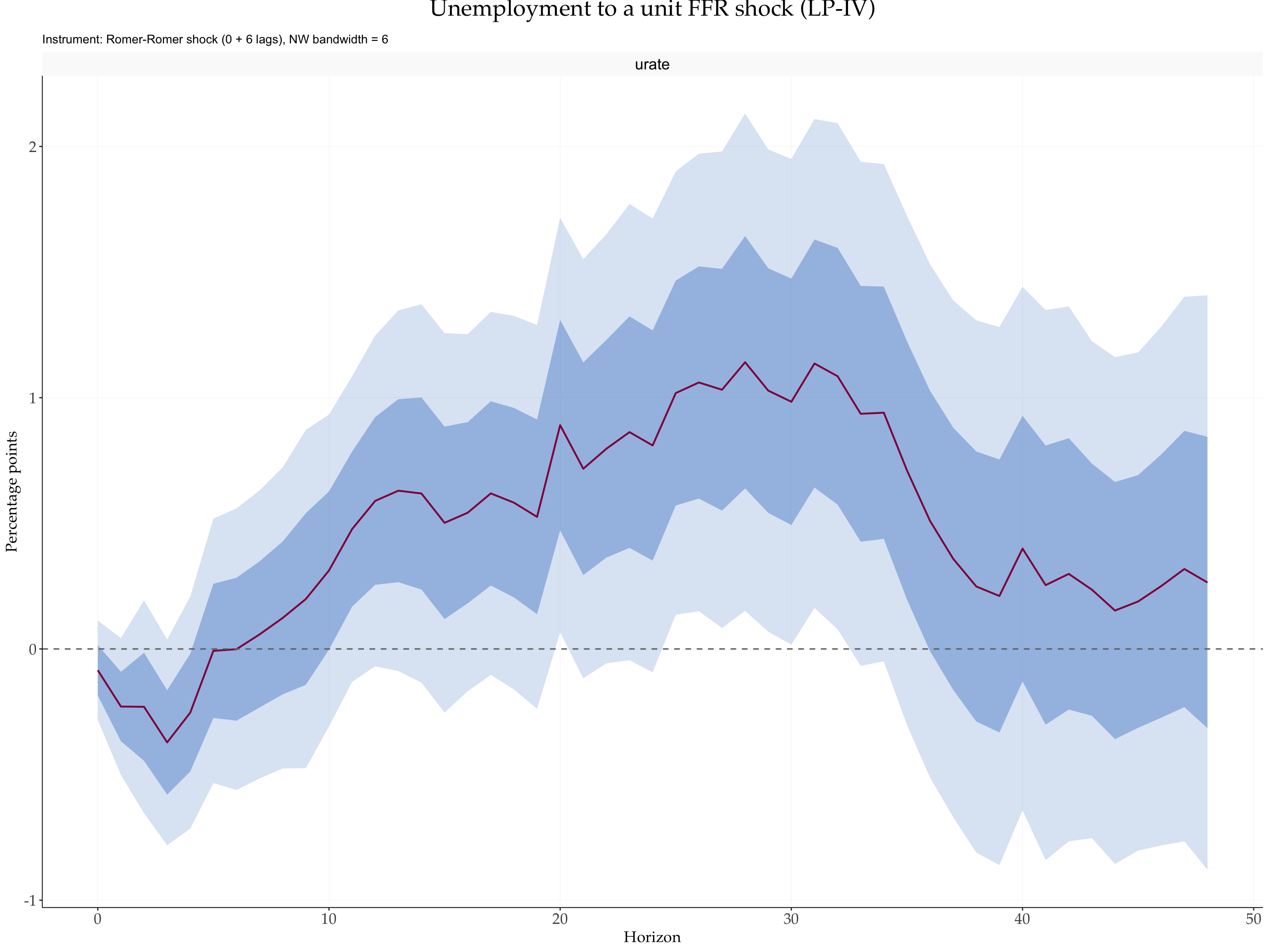

Figure 10.6: Jordà-Taylor (2025) Figure 6a: unemployment response to an FFR shock instrumented by the RR narrative shock

tibble::tibble(horizon = 0:48, F = as.numeric(lp_iv$Fstat_fs)) |>
  ggplot(aes(x = horizon, y = F)) +
    geom_col(fill = "#407EC9", alpha = 0.75) +
    geom_hline(yintercept = 10, colour = "#910048", linetype = "dashed") +
    labs(x = "Horizon", y = "First-stage F",
         title = "First-stage F across horizons")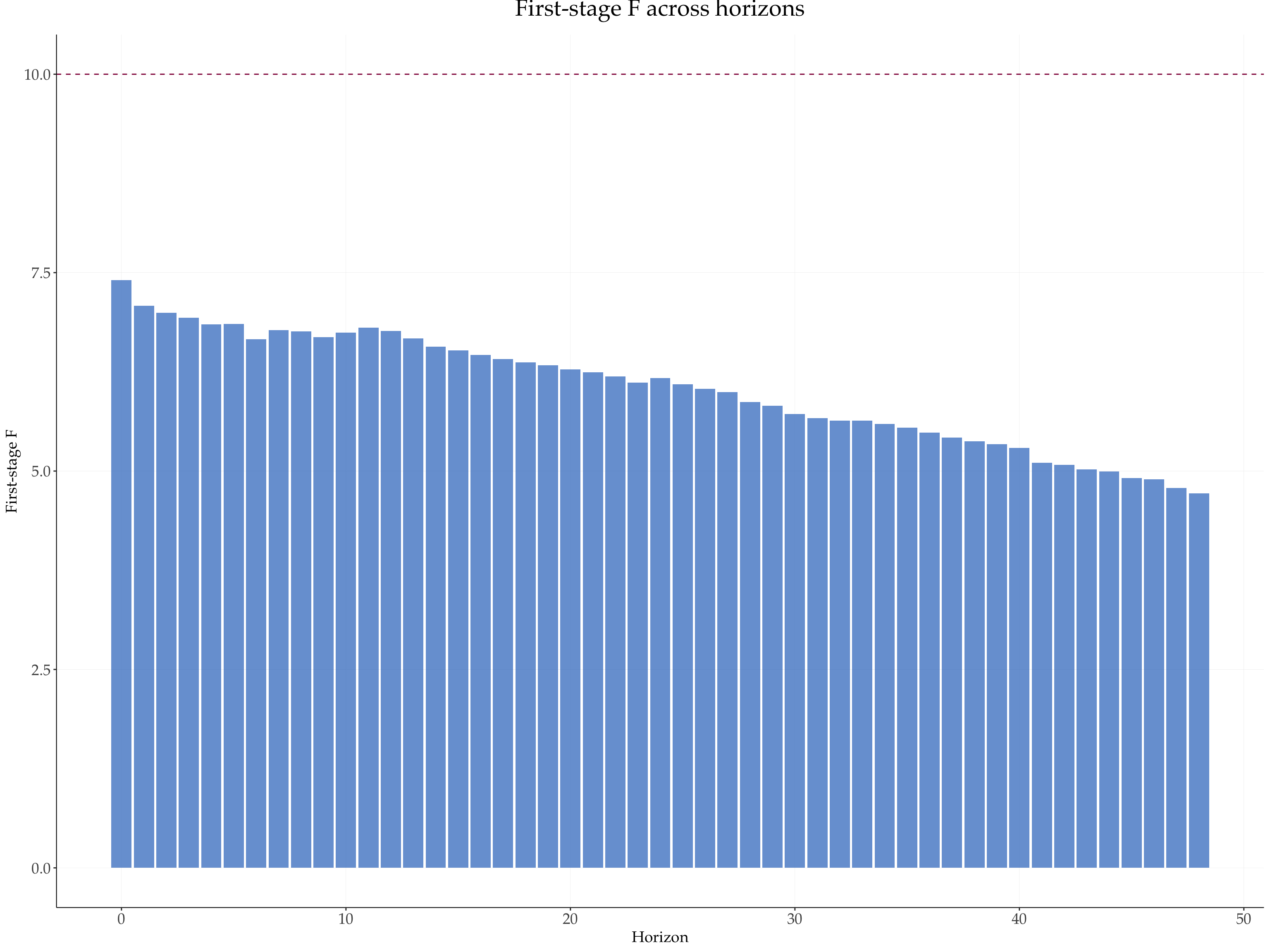

Figure 10.7: First-stage F-statistic across horizons (values below 10 flag a weak-instrument concern)

The Fstat_fs and rsqr_fs fields expose the per-horizon first-stage diagnostics for the (residualised) IV projection — worth checking whenever the point estimates look surprising. The df convention (Th - kc - nz) is documented in the syntax primer.

---

10.9 6 · Tidy output for downstream work

tidy.fLP() returns a long data frame. For single-band fits, the shape matches the historical broom-style output (estimate, se, lower, upper). For multi-band fits, one lower_X / upper_X column pair is produced per confidence level. It works on both fLP() and fLPIV() results.

tidy.fLP(lp_jt) |> head(6)
#>   horizon lhs   shock    estimate         se  lower_0.95 upper_0.95  lower_0.68
#> 1       0 CPI RRShock  0.03926033 0.06578167 -0.08966937  0.1681900 -0.02615677
#> 2       1 CPI RRShock  0.08884440 0.11743912 -0.14133205  0.3190209 -0.02794386
#> 3       2 CPI RRShock -0.02728809 0.16816012 -0.35687588  0.3022997 -0.19451625
#> 4       3 CPI RRShock -0.06389951 0.20501135 -0.46571437  0.3379153 -0.26777466
#> 5       4 CPI RRShock -0.07363836 0.24941001 -0.56247300  0.4151963 -0.32166611
#> 6       5 CPI RRShock -0.22802839 0.31100676 -0.83759044  0.3815337 -0.53731152
#>   upper_0.68
#> 1 0.10467743
#> 2 0.20563266
#> 3 0.13994007
#> 4 0.13997564
#> 5 0.17438939
#> 6 0.08125473

tidy.fLP(lp_jorda) |> head()
#>   horizon lhs   shock    estimate         se       lower     upper
#> 1       0 CPI RRShock  0.03926033 0.06578167 -0.06894088 0.1474616
#> 2       1 CPI RRShock  0.08884440 0.11743912 -0.10432577 0.2820146
#> 3       2 CPI RRShock -0.02728809 0.16816012 -0.30388688 0.2493107
#> 4       3 CPI RRShock -0.06389951 0.20501135 -0.40111317 0.2733141
#> 5       4 CPI RRShock -0.07363836 0.24941001 -0.48388132 0.3366046
#> 6       5 CPI RRShock -0.22802839 0.31100676 -0.73958899 0.2835322

tidy.fLP(lp_iv) |> head(6)
#>   horizon   lhs shock     estimate        se lower_0.95 upper_0.95 lower_0.68
#> 1       0 urate   ffr -0.084687889 0.1008886 -0.2824259 0.11305010 -0.1850173
#> 2       1 urate   ffr -0.229171350 0.1389692 -0.5015460 0.04320333 -0.3673704
#> 3       2 urate   ffr -0.230136875 0.2162507 -0.6539804 0.19370666 -0.4451891
#> 4       3 urate   ffr -0.371867562 0.2088968 -0.7812977 0.03756257 -0.5796066
#> 5       4 urate   ffr -0.253362503 0.2356595 -0.7152467 0.20852168 -0.4877160
#> 6       5 urate   ffr -0.007562491 0.2685829 -0.5339752 0.51885025 -0.2746568
#>    upper_0.68
#> 1  0.01564156
#> 2 -0.09097231
#> 3 -0.01508469
#> 4 -0.16412853
#> 5 -0.01900903
#> 6  0.25953186

---

10.10 Summary

• nw_offset = 0 (classic Jordà = h rule) and nw_lags_iv = 6 reproduce the Jorda and Taylor (2025) MATLAB / Stata standard errors.
• Both fLP() and fLPIV() handle multi-band conf and, for fLP(), multi-equation LHS in a single fit — see the syntax primer for the shared conventions.

References

Jorda, Oscar, and Alan M. Taylor. 2025. “Local Projections.” Journal of Economic Literature 63 (1): 59–110. https://doi.org/10.1257/jel.20241521.