Identification via sign restrictions and external instruments

1 Setup

library(tidyverse)
library(tidyMacro)

theme_set(fThemeTidyMacro())

# Shock 1 is instrumented; shock 2 is identified by sign restrictions.
financial_shock <- 2

2 Sign restrictions + External Instruments (IV)

The two strategies can be combined, as proposed by Cesa-Bianchi and Sokol (2022). The motivation is practical: a researcher often has a credible instrument for one shock, typically monetary policy, but nothing comparable for the others. Rather than discard the instrument or leave the remaining shocks unidentified, the instrument point-identifies its column of \(B\) and sign restrictions set-identify the rest.

Partition \(B = \begin{bmatrix} B^{IV} & B^{SR} \end{bmatrix}\). The first block is point-identified by the proxy through the usual two-stage regression (Stock and Watson 2012; Mertens and Ravn 2013): regress the first variable’s residual on the instrument, then project the remaining residuals on the fitted values to recover the ratios \(b_{i1}/b_{11}\), and rescale to shock units. The second block is set identified. The difference from plain sign restrictions is how \(Q_j\) is built: sequentially rather than by QR:

Find the unit vector \(Q^{IV}\) that rotates the first column of \(P\) into \(B^{IV}\), i.e. \(PQ^{IV} = B^{IV}\).
Given \(Q^{IV}\), complete the remaining columns by Gram-Schmidt on standard normal draws, so that \(Q_j = \begin{bmatrix} Q^{IV} & Q_j^{SR}\end{bmatrix}\) is orthonormal.

Then \(B_j = PQ_j\) satisfies \(\Sigma_u = B_jB_j'\) with its first column pinned at the IV estimate, and only the remaining columns are screened against the sign restrictions. The monetary policy shock is never touched by the rotation loop.

What the scheme looks like in its original application

Cesa-Bianchi and Sokol (2022) use sign+iv to identify a financial shock, and the shape of their design is worth knowing because it is more demanding than the illustration below.

Their US block is a five-variable monthly VAR(12) over 1979m7-2016m12 in the 1-year rate, the corporate bond yield, real GDP, the CPI and the excess bond premium. Two shocks are point-identified by external instruments, the monetary policy and central bank information surprises of Jarociński and Karadi (2020), and only one further shock is set-identified by sign restrictions. A contractionary financial shock is defined as one that lowers output, prices and the policy rate while raising the credit spread and the borrowing rate; the restriction that does the identifying work is the last one, since it is the response of the borrowing rate that separates a financial shock from an ordinary demand shock. Restrictions are imposed over three months, and inference is a wild bootstrap following Mertens and Ravn (2013) rather than the Normal-inverse-Wishart posterior used here.

fSignRestr() accepts a \(k\)-column instrument and leaves \(N-k\) columns for sign restrictions. Its inference uses posterior VAR draws with an IV block estimated once.

2.1 The uncertainty the toolbox leaves out

The IV column is recovered once on the OLS point estimate. The draw loop then redraws \((\Phi, \Sigma_u)\) from the posterior at every iteration but reads \(B^{IV}\) back from that fixed value, regardless of the inference flag. The instrument’s own sampling error, the first-stage uncertainty that weak-instrument diagnostics are about, never reaches the bands.

The VAR Toolbox keeps the first-stage estimate at OLS rather than re-estimating it during posterior draws. The covariance normalization described below still changes the impact column’s length. A joint likelihood, as in Caldara and Herbst (2019) or Arias et al. (2021), is one route to modelling instrument uncertainty. Another is resampling residuals and instruments together and re-estimating the first stage, as in the Bianchi-Sokol wild bootstrap; this does not automatically provide inference robust to weak instruments. fSignRestr() follows the toolbox, so the bands on the instrumented shock should be read as conditional on the first stage.

The fixed column is renormalised against each draw’s Cholesky factor, \(b_1 / \lVert L^{-1}b_1 \rVert\), so its direction is constant but its length is not. For multiple instruments, Gram-Schmidt also changes subsequent columns’ directions when the IV-sample and VAR-draw covariances differ. Thus “fixed” means that the first stage is not re-estimated; it does not mean that every numerical entry of the impact block is unchanged. The paper’s bootstrap uses the IV-sample covariance for both recovery and completion.

3 Pseudo-application: Cesa-Bianchi and Sokol (2022) with one instrument

This is a pseudo-application, adapted from Cesa-Bianchi and Sokol (2022), rather than a replication of their estimates. We use their US data and financial-shock sign restrictions, but retain only the monetary-policy instrument MPshockSign from Jarociński and Karadi (2020).

The differences from the paper are substantive:

The paper uses both monetary-policy and central-bank-information instruments. Here CBIshockSign is omitted, so the financial shock is constrained to be orthogonal to the instrument-identified monetary shock, without separately identifying an information shock. This changes the identification assumptions.
The paper uses a wild bootstrap that re-estimates the IV block. Here fSignRestr() uses posterior VAR draws conditional on a first-stage estimate computed once, with the covariance normalization described above. The resulting bands do not incorporate first-stage sampling uncertainty.
We illustrate only the US block, without the paper’s UK transmission model or counterfactuals.

3.1 Data and identification

The model is a five-variable monthly VAR(12) with a constant, using observations from 1979:M7 through 2016:M12. The variables are the one-year Treasury rate, corporate bond yield, real GDP, CPI and excess bond premium. CBS2022 stores GDP and CPI in logs, the two interest rates in decimal units, and EBP in percentage points. No additional log transformation is needed. Missing instrument observations remain NA; genuine zeros are retained.

data("CBS2022", package = "tidyMacro")

us <- CBS2022 |>
  filter(Date >= as.Date("1979-07-01"), Date <= as.Date("2016-12-01"))

# The first-stage normalization equation is the one-year policy rate.
y <- us |>
  select(i_1YR, BondYield, lnRGDP, CPI, EBP)

# Pseudo-application: use only the monetary-policy instrument.
z <- us |>
  select(MPshockSign)

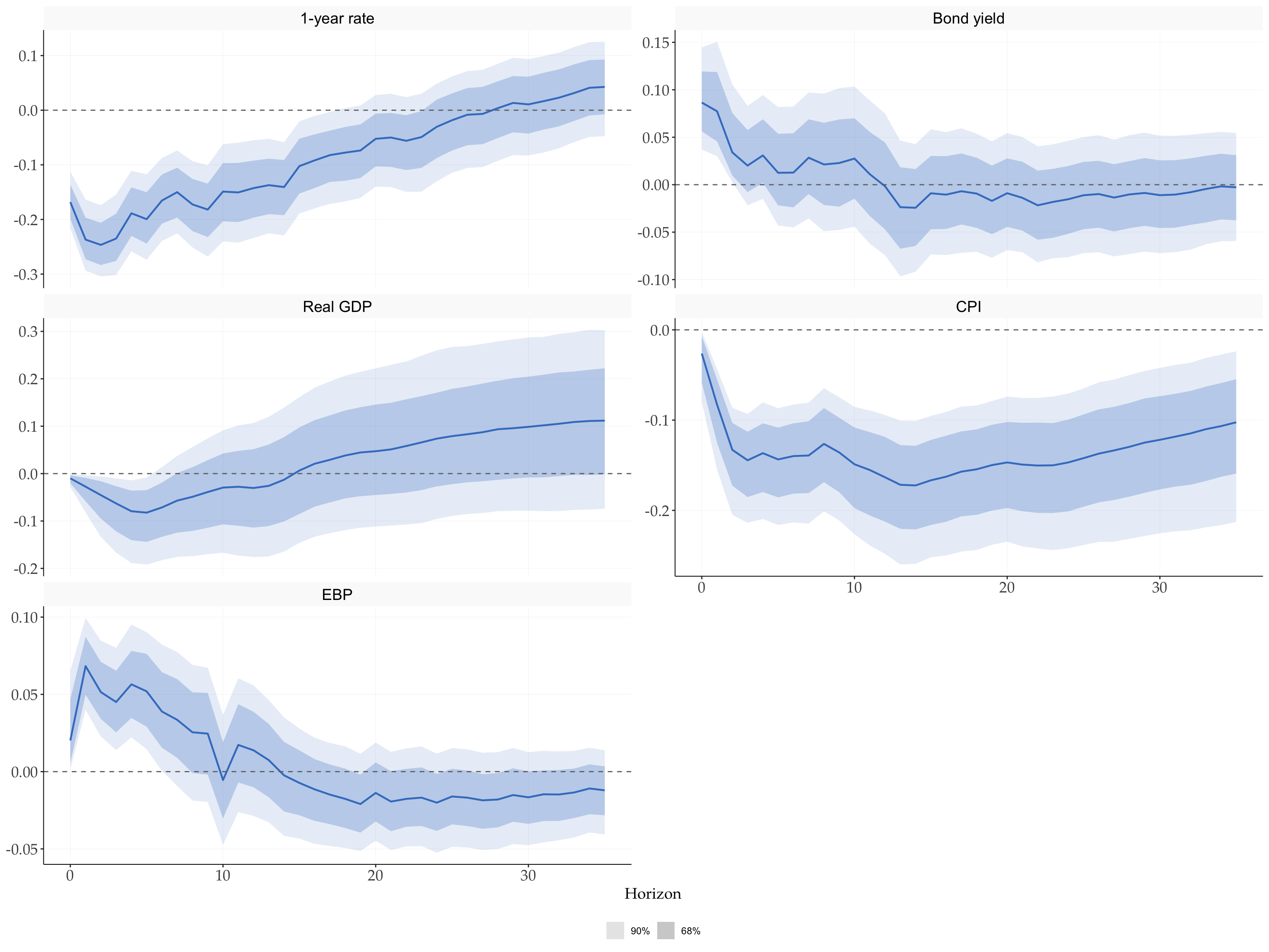
Shock 1 is identified by the instrument. Shock 2 is an adverse financial shock: it lowers the policy rate, real GDP and CPI while raising the bond yield and excess bond premium. These signs are imposed on impact and for the following two months (sr_hor = 3). The other three shocks are unrestricted. A zero in the sign matrix means unrestricted, not an exact zero response.

# With one instrument, column 1 of this 5 x 4 matrix identifies shock 2.
sign_financial <- matrix(
  0, nrow = 5, ncol = 4,
  dimnames = list(names(y), NULL)
)
sign_financial[, 1] <- c(-1, 1, -1, -1, 1)

bs_us <- fSignRestr(
  y = y,
  p = 12,
  c = 1,
  sign = sign_financial,
  instrument = list(Z = z),
  nsteps = 36,
  ndraws = 2000,
  sr_hor = 3,
  sr_rot = 1000,
  conf = c(68, 90),
  inference = 1,
  store_draws = FALSE,
  varnames = c("1-year rate", "Bond yield", "Real GDP", "CPI", "EBP"),
  seed = 2022
)

bs_us
#> Sign-restricted SVAR (sign+iv)
#>   Variables      : 1-year rate, Bond yield, Real GDP, CPI, EBP
#>   Lags           : 12   Intercept: 1
#>   Accepted draws : 2000 of 2000 slots (0 failed)
#>   Rotations tried: 84,233   acceptance: 2.374%
#>   Horizons       : 36   bands: 68, 90%
#>   Instrument     : first-stage F = 6.47, R2 = 0.020, n = 323
#>   IV column(s)   : fixed at OLS (VAR Toolbox convention)

3.2 Financial-shock responses

The figure plots shock 2, the sign-identified financial shock. Its signs over months 0–2 are imposed by construction; responses at later horizons are unrestricted. The instrument-identified monetary shock occupies column 1 and is not the shock plotted here.

fPlotIRFSign(
  bs_us,
  shock = financial_shock,
  labels = "Financial shock (single-IV pseudo-application)",
  conf = c(68, 90),
  # Convert decimal rates to percentage points and logs to percent.
  # EBP is already in percentage points.
  scale = c(100, 100, 100, 100, 1),
  facet_ncol = 2
)

Figure 1: Pseudo-application adapted from Cesa-Bianchi and Sokol (2022): responses to an adverse financial shock, conditional on a monetary shock identified by a single instrument. Median with 68% and 90% conditional credible bands. Five-variable monthly US VAR(12) with a constant, 1979:M7-2016:M12. GDP and CPI responses are in approximate percent; interest-rate and EBP responses are in percentage points.

3.3 Instrument relevance and interpretation

The first stage uses the one-year-rate residual and the observed monetary-policy instrument. The diagnostic therefore pertains to the instrumented monetary shock, not directly to the sign-identified financial shock.

iv <- bs_us[["iv"]]
tibble(
  instrument = "MPshockSign (Jarocinski-Karadi)",
  F = iv$fs_F,
  R2 = iv$fs_r2,
  n = iv$n_iv
) |>
  mutate(across(where(is.numeric), \(x) round(x, 3))) |>
  gt::gt()

instrument	F	R2	n
MPshockSign (Jarocinski-Karadi)	6.474	0.02	323

For this specification, the first-stage F-statistic is approximately 6.47, which raises a weak-instrument concern. The financial shock is identified conditional on the estimated monetary-shock direction, so uncertainty in that direction also matters for its interpretation. These conditional credible bands are not weak-instrument-robust confidence sets. The exercise demonstrates how to combine an instrument with sign restrictions; it should not be presented as reproducing the paper’s financial-shock estimates.

4 Cesa-Bianchi and Sokol (2022)

Cesa-Bianchi and Sokol (2022) reports the domestic responses to an adverse US financial shock. The model is a five-variable monthly VAR(12) with a constant, estimated from 1979:M7 through 2016:M12. The endogenous variables are ordered as the one-year Treasury rate, corporate bond yield, real GDP, CPI and the excess bond premium. Monetary policy and central-bank-information shocks are jointly identified by the two high-frequency surprises of Jarociński and Karadi (2020). Conditional on those two columns, the financial shock is the first shock left for sign identification.

The financial shock lowers the policy rate, real GDP and CPI while raising the borrowing rate and the excess bond premium. These signs hold on impact and for the following two months. The remaining demand and supply shocks are unrestricted.

For the supplied US data at the OLS estimate, the impact signs have no nonzero direction in the complement of the two IV columns. More rotations of that fixed model cannot help. The all-rotation C++ collector now checks for a well-conditioned linear certificate of this incompatibility in small free subspaces, returning infeasible = TRUE, n_tried = 0 and the excluded rotation budget in n_ruled_out. Every bootstrap VAR must be checked separately: this OLS finding is not a claim that the entire bootstrap has no admissible models.

4.1 Replication code

data("CBS2022", package = "tidyMacro")

us <- CBS2022 |>
  dplyr::filter(Date >= as.Date("1979-07-01"), Date <= as.Date("2016-12-01"))

y <- us |>
  select(i_1YR, BondYield, lnRGDP, CPI, EBP)

z <- us |>
  select(MPshockSign, CBIshockSign)

# Shocks 1 and 2 are identified by the instruments. Column 1 identifies
# shock 3, the adverse financial shock; demand and supply remain unrestricted.
sign_financial      <- matrix(0, nrow = 5, ncol = 3)
sign_financial[, 1] <- c(-1, 1, -1, -1, 1)

bs_us <- fSignRestr(
    y = y,
    p = 12,
    c = 1,
    sign = sign_financial,
    instrument = list(Z = z),
    nsteps = 36,
    ndraws = 2000,
    sr_hor = 3,
    sr_rot = 10000,
    conf = c(68, 90),
    store_draws = FALSE,
    varnames    = c("1-year rate", "Bond yield", "Real GDP", "CPI", "EBP"),
    seed = 2022
)

fPlotIRFSign(
  bs_us,
  shock = 3,
  labels = "Financial shock",
  conf = c(68, 90),
  scale = 100,
  facet_ncol = 3
)

5 References

Arias, Jonas E., Juan F. Rubio-Ramírez, and Daniel F. Waggoner. 2021. “Inference in Bayesian Proxy-SVARs.” Journal of Econometrics 225 (1): 88–106.

Caldara, Dario, and Edward Herbst. 2019. “Monetary Policy, Real Activity, and Credit Spreads: Evidence from Bayesian Proxy SVARs.” American Economic Journal: Macroeconomics 11 (1): 157–92.

Cesa-Bianchi, Ambrogio, and Andrej Sokol. 2022. “Financial Shocks, Credit Spreads, and the International Credit Channel.” Journal of International Economics 135: 103543. https://doi.org/10.1016/j.jinteco.2021.103543.

Jarociński, Marek, and Peter Karadi. 2020. “Deconstructing Monetary Policy Surprises: The Role of Information Shocks.” American Economic Journal: Macroeconomics 12 (2): 1–43. https://doi.org/10.1257/mac.20180090.

Mertens, Karel, and Morten O. Ravn. 2013. “The Dynamic Effects of Personal and Corporate Income Tax Changes in the United States.” American Economic Review 103 (4): 1212–47.

Stock, James H., and Mark W. Watson. 2012. “Disentangling the Channels of the 2007-09 Recession.” Brookings Papers on Economic Activity 43 (1): 81–135.