6  Internal Instruments: Cholesky on Augmented VAR

Oil Supply News with the Instrument Ordered First (Kaenzig 2021)

6.1 Overview

Following Plagborg-Møller and Wolf (2021), the same oil supply news shock as in Känzig (2021) can be identified recursively by adding the instrument to the VAR as the first variable and applying a Cholesky decomposition. Under invertibility, the internal-instrument IRFs are asymptotically equivalent to the proxy-SVAR IRFs; the price is estimating the reduced-form VAR on the (shorter) sample for which the instrument is observed.

6.2 Setup

library(tidyverse)
library(tidyMacro)
library(tictoc)

set_theme(fThemeTidyMacro())

---

6.3 Data

The instrument is missing outside the OPEC-announcement window; per the original paper we truncate the missing values to zero so that the augmented VAR can be estimated on the full sample.

data("Kaenzig2021")

finaldata <- Kaenzig2021 |>
    select(Oil_Price, World_Oil_Prod, World_Oil_Inven, World_IP, US_IP, US_CPI) |>
    as.matrix()

iv_oil_trunc <- Kaenzig2021 |>
    select(iv_kanzig_final) |>
    mutate(iv_kanzig_final = ifelse(is.na(iv_kanzig_final), 0, iv_kanzig_final)) |>
    as.matrix()

varnames     <- c("Oil Price", "World Oil Prod.", "World Oil Inven.",
                  "World IP", "US IP", "US CPI")
varnames_aug <- c("Oil Instrument", varnames)

6.4 Augmented VAR and Cholesky IRF

p <- 12
c <- 1
hor <- 48

y_aug <- cbind(iv_oil_trunc, finaldata)

var_aug  <- fVAR(y_aug, p, c)
S_aug    <- t(chol(var_aug$sigma))
wold_aug <- fWoldIRF(var_aug, horizon = hor)

point_irf_aug <- fCholeskyIRF(wold_aug, S_aug)

6.5 Bootstrap

tic()
boot_aug <- fBootstrapChol(
    y          = y_aug,
    var_result = var_aug,
    nboot      = 1000,
    horizon    = hor,
    prc        = 90,
    prc2       = 68,
    n_threads  = 3
)
toc()
#> 1.762 sec elapsed

6.6 Impulse Response Functions

Responses are rescaled so that the impact on the oil price matches a 10% jump, mirroring the proxy-SVAR scale.

# point_irf_aug[2, 1, 1]: oil price (row 2), shock 1, h = 0
scale_int <- 10 / point_irf_aug[2, 1, 1]

fPlotIRFChol(
    point       = point_irf_aug,
    boot_result = boot_aug,
    shock       = 1,
    varnames    = varnames_aug,
    facet_ncol  = 3,
    return_data = TRUE
) |>
  filter(variable != "Oil Instrument") |>
  mutate(
    variable = factor(variable, levels = varnames),
    across(c(point, upper, lower, upper2, lower2), ~ . * scale_int)
  ) |>
  ggplot(aes(x = horizon)) +
  geom_ribbon(aes(ymin = lower,  ymax = upper),  fill = "#407EC9", alpha = 0.20) +
  geom_ribbon(aes(ymin = lower2, ymax = upper2), fill = "#407EC9", alpha = 0.35) +
  geom_line(aes(y = point), color = "#910048", linewidth = 0.8) +
  geom_hline(yintercept = 0, linetype = "dashed", color = "#707372", linewidth = 0.6) +
  facet_wrap(~ variable, scales = "free", ncol = 3) +
  labs(x = NULL, y = NULL)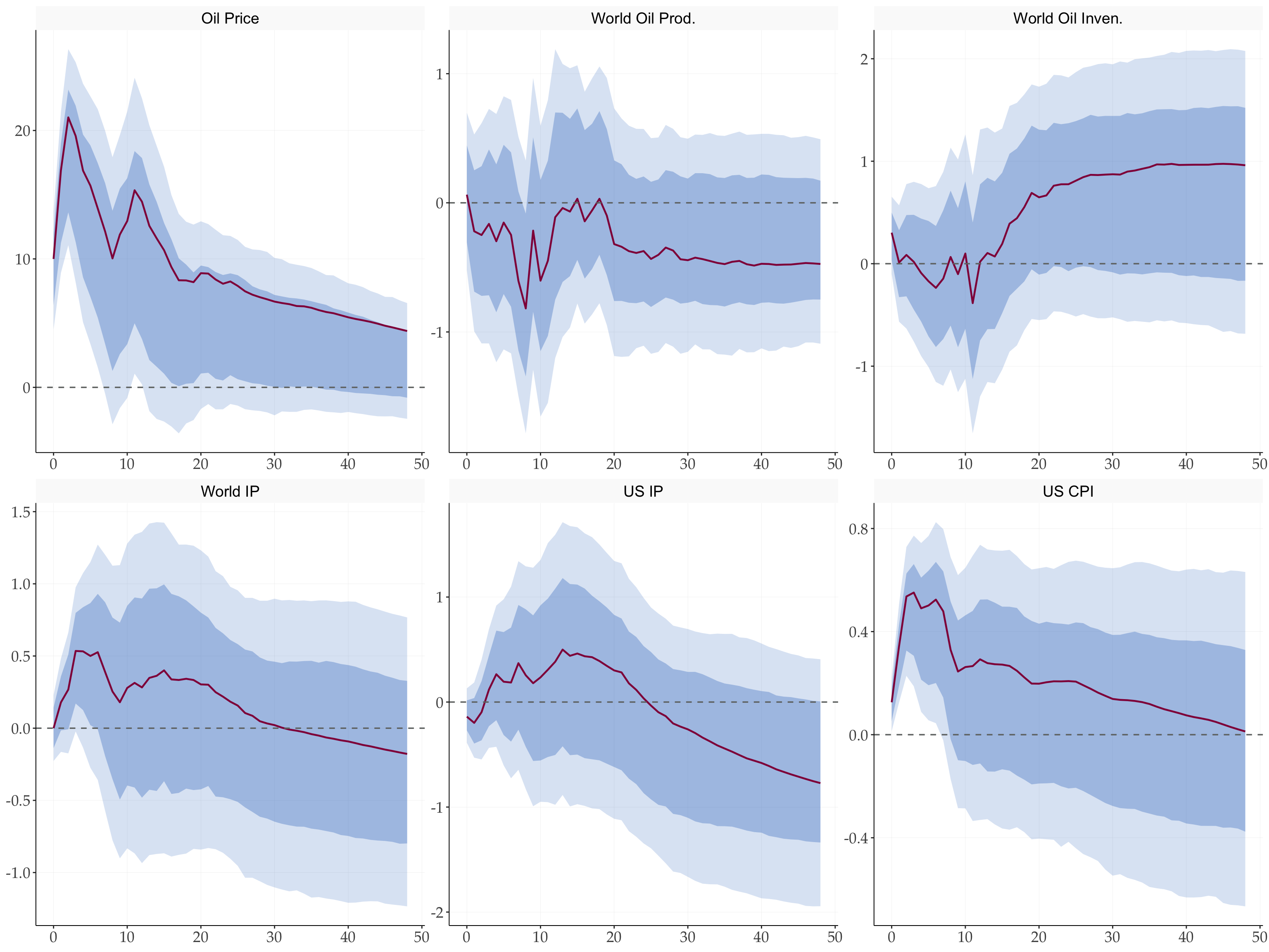

Figure 6.1: IRFs to oil supply news shock — internal instruments (Cholesky, 68% and 90% confidence bands). Units: 10% impact on the oil price.

One should read these results with care: unlike proxy-SVAR, the augmented VAR is estimated on the shorter sample for which the instrument is observed, so tail-end coverage is thinner.

References

Känzig, Diego R. 2021. “The Macroeconomic Effects of Oil Supply News: Evidence from OPEC Announcements.” American Economic Review 111 (4): 1092–125. https://doi.org/10.1257/aer.20190964.

Plagborg-Møller, Mikkel, and Christian K. Wolf. 2021. “Local Projections and VARs Estimate the Same Impulse Responses.” Econometrica 89 (2): 955–80. https://doi.org/10.3982/ECTA17813.