5  Proxy SVAR (External Instruments) and Weak-IV Robust Inference

The Macroeconomic Effects of Oil Supply News: Evidence from OPEC Announcements

5.1 Overview

This document replicates the main empirical results of Känzig (2021), which identifies oil supply news shocks using a high-frequency external instrument (proxy SVAR). The instrument captures exogenous variation in oil supply driven by OPEC production decisions, measured as oil futures price changes in a narrow window around OPEC announcements.

5.2 Model and Identification

Ordering the shock of interest first, a valid instrument \(z_t\) satisfies relevance and exogeneity:

\[\mathbb{E}[z_t \varepsilon_{1t}] = \alpha \neq 0, \qquad \mathbb{E}[z_t \varepsilon_{kt}] = 0, \quad k = 2, \dots, K.\]

These conditions imply \(\mathbb{E}[z_t u_t] = \alpha\, b_1\), so the impact column is recovered up to scale from covariance ratios (a two-stage regression of the residuals on \(z_t\)):

\[\frac{b_{i1}}{b_{11}} = \frac{\mathbb{E}[z_t u_{it}]}{\mathbb{E}[z_t u_{1t}]}, \qquad \Theta_h = \Phi_h\, b_1.\]

---

5.3 Setup

library(tidyverse)
library(tidyMacro)
library(tictoc)

set_theme(fThemeTidyMacro())

---

5.4 Data

data("Kaenzig2021")

finaldata <- Kaenzig2021 |>
    select(Oil_Price, World_Oil_Prod, World_Oil_Inven, World_IP, US_IP, US_CPI) |>
    as.matrix()

iv_oil <- Kaenzig2021 |>
    select(iv_kanzig_final) |>
    drop_na() |>
    as.matrix()

# Truncated to zero (used for instrument-strength diagnostics only)
iv_oil_trunc <- Kaenzig2021 |>
    select(iv_kanzig_final) |>
    mutate(iv_kanzig_final = ifelse(is.na(iv_kanzig_final), 0, iv_kanzig_final)) |>
    as.matrix()

N         <- ncol(finaldata)
varnames  <- c("Oil Price", "World Oil Prod.", "World Oil Inven.",
               "World IP", "US IP", "US CPI")
shockname <- "Oil Shock"

5.5 VAR Estimation

p <- 12
c <- 1

var_result <- fVAR(finaldata, p, c)
beta       <- var_result$beta
residuals  <- var_result$residuals
sigma_full <- var_result$sigma

hor  <- 48
wold <- fWoldIRF(var_result, horizon = hor)

5.6 Proxy SVAR: MBB Bootstrap

adjustZ <- c(1, nrow(iv_oil))
adjustu <- c(nrow(residuals) - nrow(iv_oil) + 1, nrow(residuals))

tic()
result_mbb <- fBootstrapIVMBB(
    y          = finaldata,
    var_result = var_result,
    Z          = iv_oil,
    nboot      = 1000,
    blocksize  = 24,          # 0: auto block size, 24 is in the paper
    adjustZ    = adjustZ,
    adjustu    = adjustu,
    policyvar  = 1,
    horizon    = hor,
    n_threads  = 3
)
#> Using 3 thread(s) for parallel bootstrap computation...
toc()
#> 1.166 sec elapsed

5.7 Impulse Response Functions

fPlotIRFIV(
    result_mbb = result_mbb,
    varnames   = varnames,
    shockname  = shockname,
    scale      = 10,
    facet_ncol = 3
) +
  labs(x = NULL, y = NULL)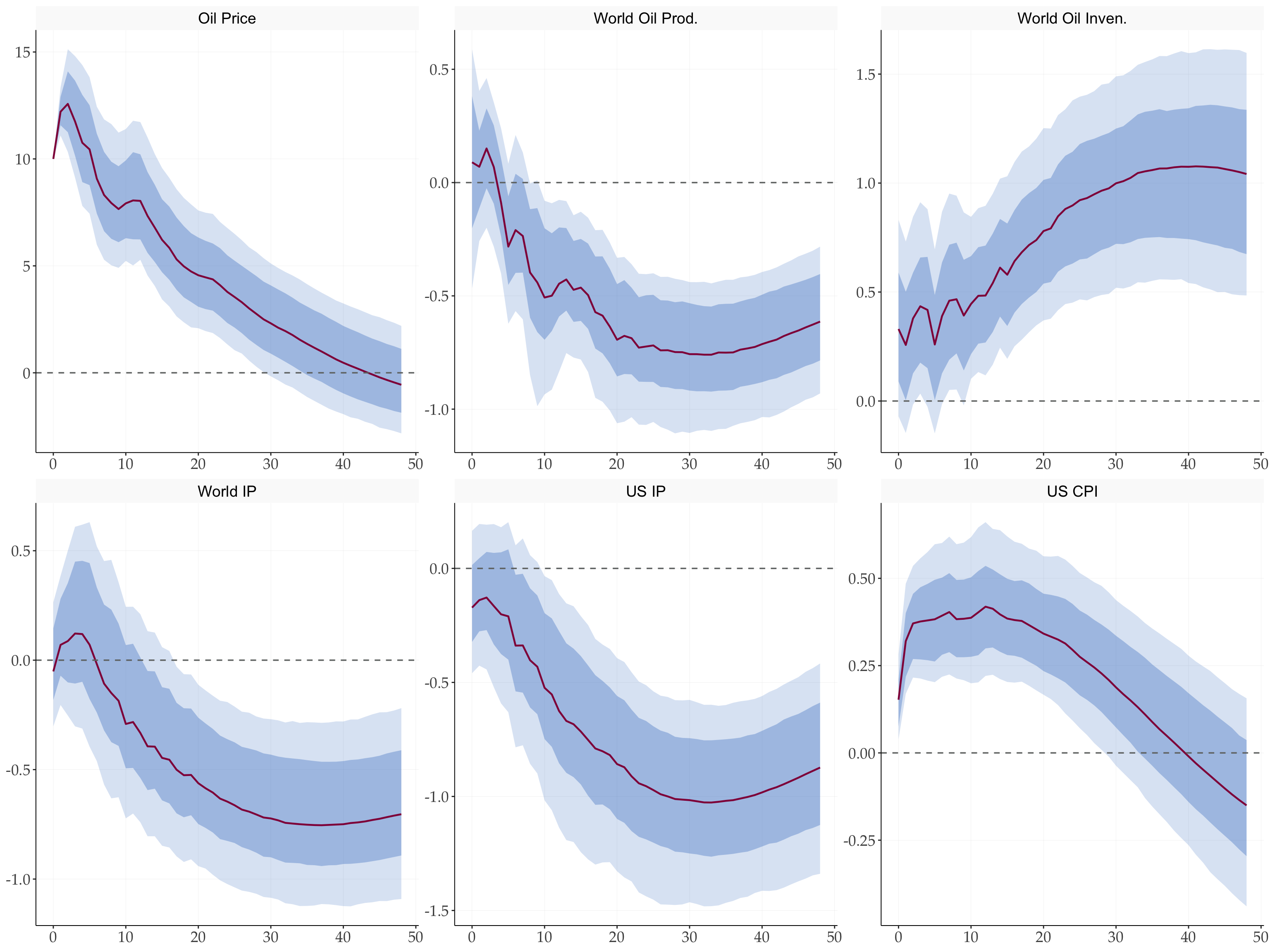

Figure 5.1: IRFs to oil supply news shock — MBB bootstrap (68% and 90% confidence bands)

5.8 Instrument Strength

u_p <- residuals[, 1]

# Match the paper: truncate missing values to zero
iv_trunc_aligned <- tail(iv_oil_trunc, length(u_p))

strength_trunc <- fOLS(y = as.matrix(u_p), X = iv_trunc_aligned, c = 1)

# Without truncation: restrict to proxy sample only
u_p_fin  <- u_p[(length(u_p) - nrow(iv_oil) + 1):length(u_p)] |> as.matrix()
strength <- fOLS(y = u_p_fin, X = iv_oil, c = 1)

library(gt)

tibble(
    Statistic = c("F-stat", "Robust F-stat", "R²", "Adj. R²"),
    `Truncated (paper)` = c(strength_trunc$F, strength_trunc$Frobust,
                             strength_trunc$r2, strength_trunc$r2adj),
    `Without truncation` = c(strength$F, strength$Frobust,
                              strength$r2, strength$r2adj)
) |>
  gt() |>
  fmt_number(columns = 2:3, decimals = 3) |>
  tab_header(title = "First-Stage Instrument Strength") |>
  tab_footnote("Rule of thumb: F-stat > 10 indicates a strong instrument.")

First-Stage Instrument Strength
Statistic	Truncated (paper)	Without truncation
F-stat	22.669	20.259
Robust F-stat	10.551	10.545
R²	0.042	0.047
Adj. R²	0.040	0.044
Rule of thumb: F-stat > 10 indicates a strong instrument.

5.9 IV Identification (Manual Two-Stage)

u     <- residuals[(nrow(residuals) - length(iv_oil) + 1):nrow(residuals), ]
T1    <- nrow(u)
sigma <- (t(u) %*% u) / (T1 - 1 - p - N * p)
S     <- t(chol(sigma))

# Stage 1: regress u_p on instrument
ols1 <- fOLS(y = u_p_fin, X = iv_oil, c = 0)
uhat <- ols1$fitted_partial

# Stage 2: regress other residuals on uhat to get s_q / s_p
u_q_fin <- u[(nrow(u) - nrow(iv_oil) + 1):nrow(u), -1]
sq_sp   <- solve(t(uhat) %*% uhat) %*% t(uhat) %*% u_q_fin

# Structural impact vector (normalised to unit oil price response)
s <- c(1, sq_sp[1], sq_sp[2], sq_sp[3], sq_sp[4], sq_sp[5])

5.10 Get the Structural Shock

oil_shock <- fGetShock(
    residuals  = residuals,
    sigma_full = sigma_full,
    s          = s,
    normalize  = 'unit',
    shockSize  = 1 # for 10% use 0.1 to match Kaenzig (2021)
)

5.11 Historical Decomposition

hd_result <- fHDIV(
    residuals = residuals,
    sigma     = sigma_full,
    s         = s,
    beta      = beta,
    c         = c,
    p         = p
)
HDshock <- hd_result$HDshock

5.12 Bootstrap Uncertainty Bands for Historical Decomposition

tic()
boot_hd <- fBootstrapHDIV(
    y          = finaldata,
    var_result = var_result,
    Z          = iv_oil,
    s          = s,
    nboot      = 500L,
    blocksize  = 24L,
    adjustZ    = adjustZ,
    adjustu    = adjustu,
    policyvar  = 1L,
    prc        = 90,
    n_threads  = 3
)
#> Using 3 thread(s) for bootstrap HD computation...
toc()
#> 1.096 sec elapsed

HD1_upper <- boot_hd$upper[, 1]
HD1_lower <- boot_hd$lower[, 1]

# Date sequence aligned with VAR residuals sample (1975M01–2017M12)
dates <- seq(as.Date("1975-01-01"), as.Date("2017-12-01"), by = "month")

oil_events <- as.Date(c(
    "1978-09-01", "1980-10-01", "1985-12-01", "1990-08-01",
    "1997-07-01", "2002-11-01", "2008-09-01", "2014-11-01"
))

oil_event_labels <- c(
    "Iranian\nrevolution", "Iran-Iraq\nwar", "OPEC\ncollapse",
    "Gulf war", "Asian fin.\ncrisis", "Venezuelan\ncrisis",
    "Global fin.\ncrisis", "Oil crash\n2014"
)

hd_mean   <- mean(HDshock[, 1])
y_oil_dm  <- finaldata[(p + 1):nrow(finaldata), 1] - mean(finaldata[(p + 1):nrow(finaldata), 1])
hd_oil_dm <- HDshock[, 1] - hd_mean
upper_dm  <- HD1_upper - hd_mean
lower_dm  <- HD1_lower - hd_mean

tibble(
    date   = dates,
    actual = y_oil_dm,
    hd     = hd_oil_dm
) |>
  pivot_longer(c(actual, hd), names_to = "series", values_to = "value") |>
  mutate(series = factor(series, levels = c("actual", "hd"),
                         labels = c("Real oil price", "Contribution oil supply news"))
  ) |>
  ggplot(aes(x = date, y = value, colour = series, linetype = series)) +
  geom_ribbon(data = tibble(date = dates, lower = lower_dm, upper = upper_dm),
                aes(x = date, ymin = lower, ymax = upper),
                inherit.aes = FALSE, fill = tidyMacro_colors[3], alpha = 0.2) +
  geom_vline(xintercept = oil_events, linewidth = 0.6, colour = "grey90") +
  annotate(
    "text", x = oil_events, y = 148,
    label = oil_event_labels, size = 3.5, vjust = 1,
    colour = "grey30", lineheight = 0.85
  ) +
  geom_line(linewidth = 0.7) +
  scale_colour_manual(
    values = c("Real oil price" = tidyMacro_colors[4],
               "Contribution oil supply news" = tidyMacro_colors[1])
  ) +
  scale_x_date(date_breaks = "5 years", date_labels = "%Y") +
  ylim(-150, 150) +
  labs(x = NULL, y = "%") +
  fThemeTidyMacro()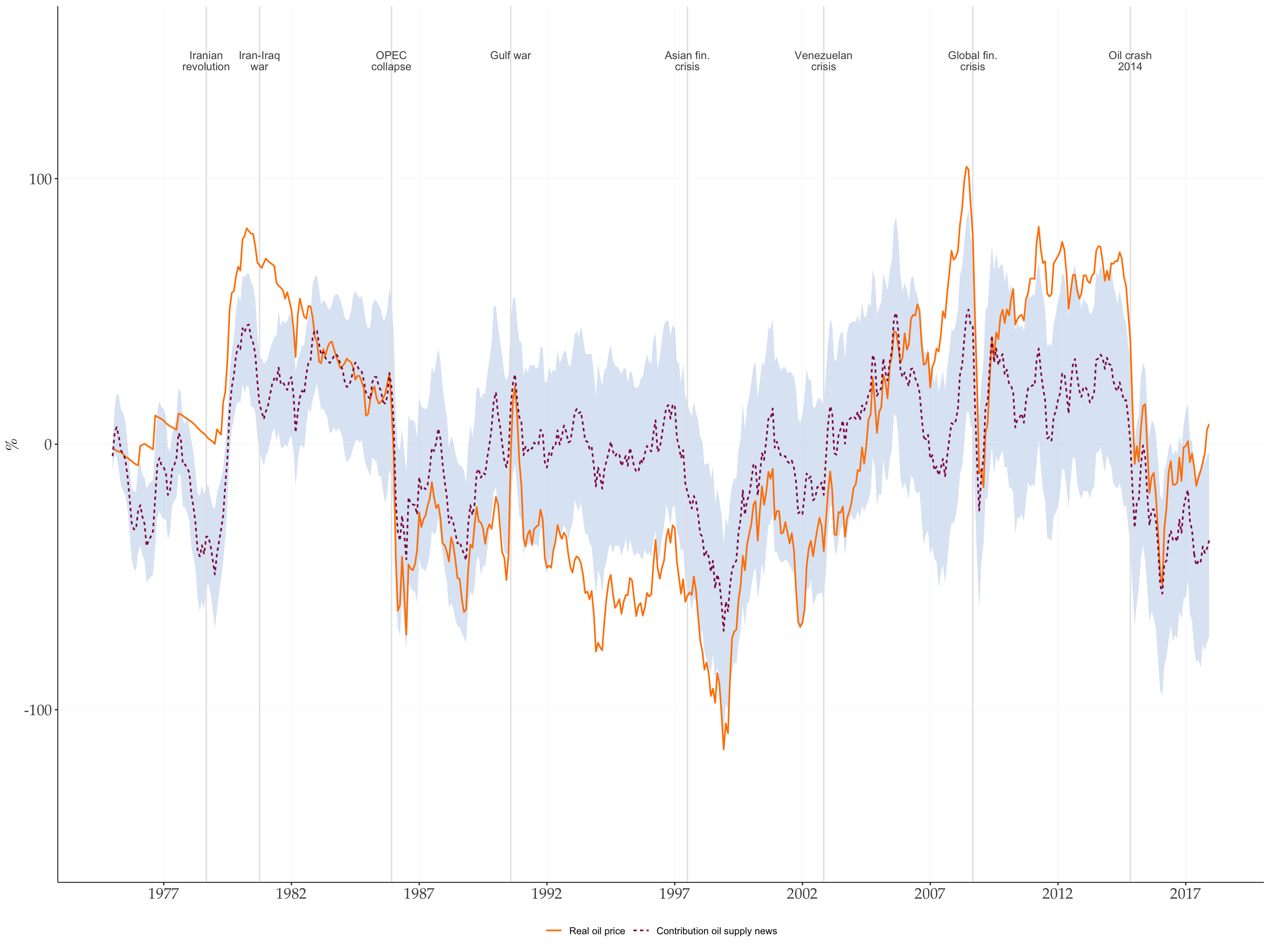

Figure 5.2: Historical decomposition: contribution of oil supply news shock to real oil price

5.13 Forecast Error Variance Decomposition

fevd_result <- fFEVDIV(s, S, wold, N, hor, sigma, u, T1 = T1, p = p)

fPlotVarDec(
    fevd       = fevd_result$fFEVDIV,
    varnames   = varnames,
    shocknames = shockname
) +
  scale_fill_manual(values = tidyMacro_colors[c(2, 4)])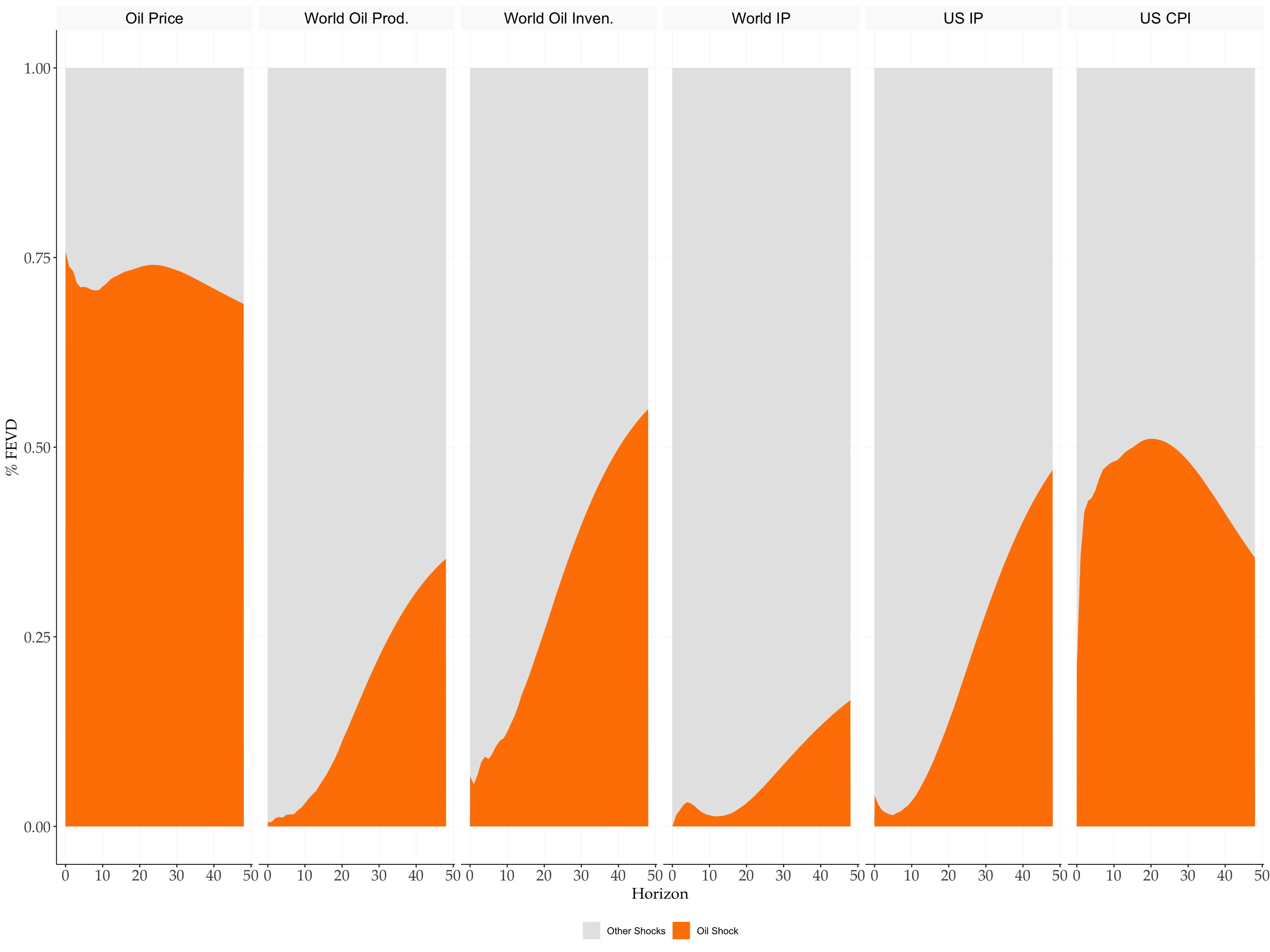

Figure 5.3: Forecast error variance decomposition: share explained by oil supply news shock

---

5.14 Weak-IV Robust Inference (Montiel-Olea, Stock, Watson 2021)

The MBB bootstrap assumes a strong instrument. Montiel Olea et al. (2021) provide confidence sets that remain valid regardless of instrument strength. Two types are reported:

• Delta method (inner, darker band): plug-in inference using the asymptotic variance of the IV estimator.
• Anderson-Rubin (outer, lighter band): weak-IV robust confidence set; bounds solve a quadratic inequality and may be unbounded if the instrument is very weak.

msw <- fMSW(
    var_result = var_result,
    Z          = iv_oil,
    finaldata  = finaldata,
    adjustu    = adjustu,
    hor        = hor,
    nvar       = 1,
    scale      = 1,
    confidence = 0.9,
    NWlags     = 0
)

cat("Wald statistic (HAC-robust F):", round(msw$Waldstat, 2), "\n")
#> Wald statistic (HAC-robust F): 11.67

fPlotIRFMSW(
    msw_result      = msw,
    varnames        = varnames,
    shockname       = shockname,
    scale           = 10,
    facet_ncol      = 3,
    line_color      = 'black',
    ribbon_fill_ar  = tidyMacro_colors[1],
    ribbon_fill_dm  = tidyMacro_colors[3],
    ribbon_alpha_ar = 0.45,
    ribbon_alpha_dm = 0.45
) +
  labs(x = NULL, y = NULL)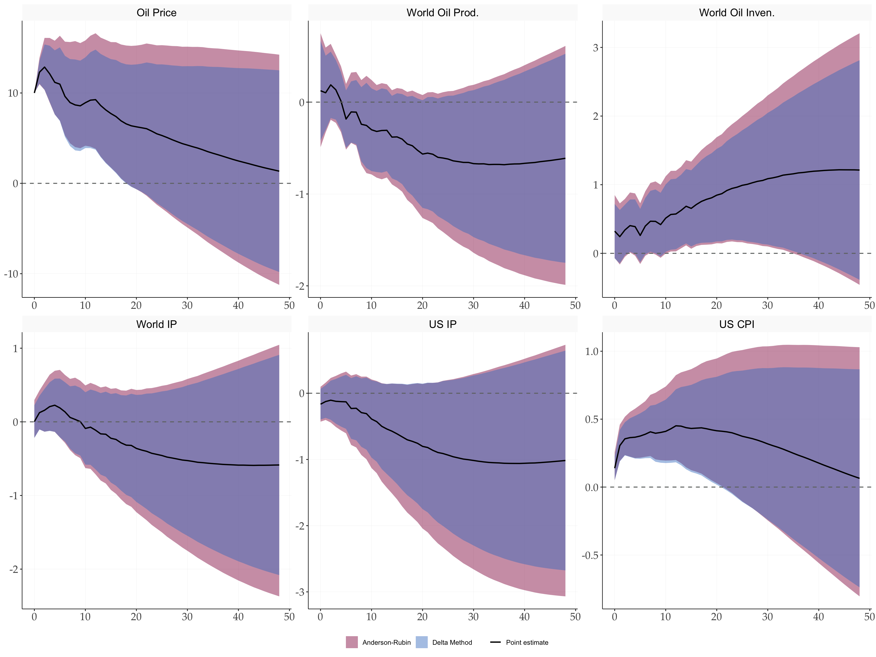

Figure 5.4: Weak-IV robust IRFs — Anderson-Rubin (outer) and delta-method (inner) 90% bands

References

Känzig, Diego R. 2021. “The Macroeconomic Effects of Oil Supply News: Evidence from OPEC Announcements.” American Economic Review 111 (4): 1092–125. https://doi.org/10.1257/aer.20190964.

Montiel Olea, José L., James H. Stock, and Mark W. Watson. 2021. “Inference in Structural Vector Autoregressions Identified with an External Instrument.” Journal of Econometrics, Themed Issue: Vector Autoregressions, vol. 225 (1): 74–87. https://doi.org/10.1016/j.jeconom.2020.05.014.