4  Mixed restrictions

News-Driven Business Cycles: Insights and Challenges

4.1 Overview

This document replicates the news shock identification of Beaudry and Portier (2014) . A news shock is identified as the shock that has no contemporaneous effect on TFP but maximizes the long-run response of TFP at a 40-quarter horizon. The approach follows the mixed restriction strategy combining a zero impact restriction with a long-run maximization criterion.

4.2 Model and Identification

With \(P\) the lower Cholesky factor of \(\Sigma\), any rotation is observationally equivalent:

\[\Sigma = P P' = (P Q)(P Q)', \qquad Q Q' = I_K.\]

The news shock is the rotation vector \(q\) orthogonal to the impact on TFP (variable 1) that maximizes the share of TFP’s forecast error variance up to horizon \(H\):

\[q^{*} = \arg\max_{q\,:\,q'q = 1,\ (Pq)_1 = 0} \frac{\sum_{h=0}^{H} \big[(\Phi_h P q)_1\big]^2}{\sum_{h=0}^{H} \sigma_{11,h}}, \qquad H = 40,\]

where \(\sigma_{11,h}\) is the total forecast error variance of TFP at horizon \(h\). The impact vector is \(b^{news} = P q^{*}\) and structural IRFs are \(\Theta_h = \Phi_h P q^{*}\).

4.3 Setup

library(tidyverse)
library(tictoc)
library(tidyMacro)

set_theme(fThemeTidyMacro())

4.4 Data

data("BeaudryPortier2014")

y        <- BeaudryPortier2014 |> as.matrix()
T_obs    <- nrow(y)
N        <- ncol(y)
varnames <- colnames(y)

4.5 VAR Estimation

p <- 2
c <- 1

var_result <- fVAR(y, p = p, c = c)
Sigma <- var_result$sigma

4.6 News Shock Identification

horizon <- 40

# Wold IRFs by inverting (I - A(L))
wold <- fWoldIRF(var_result, horizon = horizon)

# Lower Cholesky factor of Sigma
S <- t(chol(Sigma))

# LR-Max point estimate
struct_irf <- fMaxIRF(wold, S, var_idx = 1L)

4.7 Bootstrap Confidence Bands

tic()
boot_max <- fBootstrapMaxCorrected(
  y          = y,
  var_result = var_result,
  nboot1     = 1000,
  nboot2     = 2000,
  horizon    = horizon,
  var_idx    = 1,          # maximise long-run effect on TFP (variable 1)
  cumulate   = integer(0), # no cumulation (levels data)
  prc        = 68          # Match original paper
)
toc()
#> 0.265 sec elapsed

fPlotIRFLR(
  point       = struct_irf,
  boot_result = boot_max,
  varnames    = varnames,
  facet_ncol  = 2
) + labs(y  = NULL)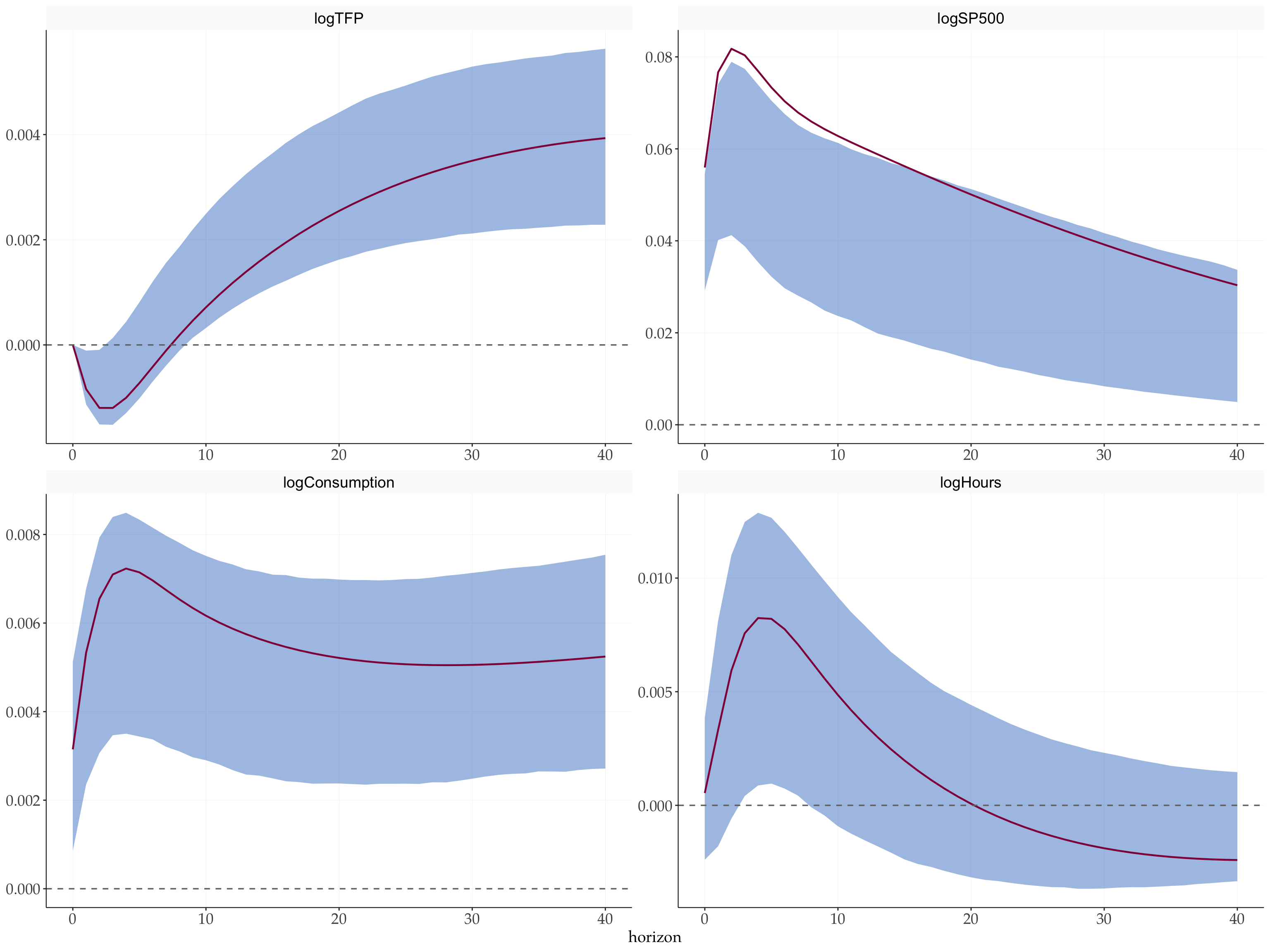

Figure 4.1: IRF to Tech. news shock — LR-Max bootstrap (68% and 90% confidence bands)

4.8 Compare the result to Barsky and Sims (2012)

Now we can compare the results to that of Barsky and Sims (2012) and plot IRF results.

struct_irf_uhlig <- fUhligIRF(wold, S, idx = 1L)

tic()
boot_uhlig <- fBootstrapUhligCorrected(
  y          = y,
  var_result = var_result,
  nboot1     = 1000,
  nboot2     = 2000,
  horizon    = horizon,
  idx        = 1L,        # maximise FEV share of TFP (variable 1)
  cumulate   = integer(0),
  prc        = 68         # Match original study
)
toc()
#> 0.286 sec elapsed

fPlotIRFLR(
  point       = struct_irf_uhlig,
  boot_result = boot_uhlig,
  varnames    = varnames,
  facet_ncol  = 2
) + labs(y  = NULL)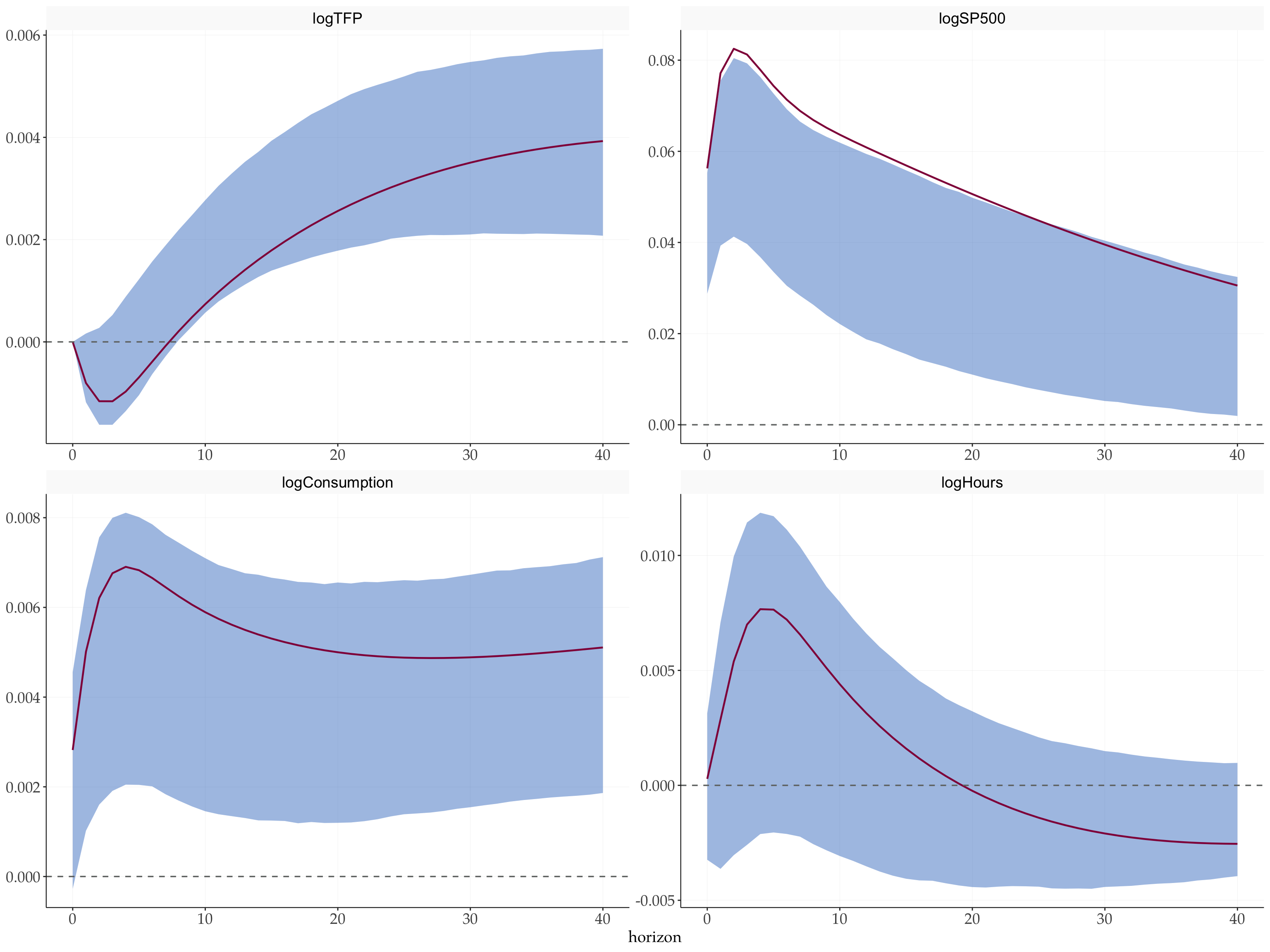

Figure 4.2: IRF to news shock — Uhlig max-share bootstrap (68% and 90% confidence bands)

References

Barsky, Robert B., and Eric R. Sims. 2012. “Information, Animal Spirits, and the Meaning of Innovations in Consumer Confidence.” American Economic Review 102 (4): 1343–77. https://doi.org/10.1257/aer.102.4.1343.

Beaudry, Paul, and Franck Portier. 2014. “News-Driven Business Cycles: Insights and Challenges.” Journal of Economic Literature 52 (4): 993–1074. https://doi.org/10.1257/jel.52.4.993.