2  Short run restrictions

The Impact of Uncertainty Shocks

2.1 Overview

This document replicates the main empirical results of Bloom (2009), which identifies uncertainty shocks using short run / recursive techniques. Data set (in all other replications as well) already come cleaned and transformed. What you see for example as x is \(log(x) * 100\)

2.2 Model and Identification

Reduced-form VAR(\(p\)):

\[y_t = c + A_1 y_{t-1} + \cdots + A_p y_{t-p} + u_t, \qquad u_t \sim (0, \Sigma)\]

Structural shocks: \(u_t = B_0 \varepsilon_t\) with \(\varepsilon_t \sim (0, I_K)\), so the data only pin down

\[\Sigma = B_0 B_0'.\]

Recursive (Cholesky) identification sets the upper triangle of \(B_0\) to zero:

\[\Sigma = P P', \qquad B_0 = P \ \text{(lower triangular)}.\]

Structural IRFs from the Wold coefficients \(\Phi_h\):

\[\Theta_h = \Phi_h B_0, \qquad h = 0, 1, \dots, H.\]

2.3 Setup

library(tidyverse)
library(tidyMacro)
library(tictoc)

set_theme(fThemeTidyMacro())

---

2.4 Data

data("Bloom2009")

# See Data
Bloom2009 |> head()
#> # A tibble: 6 × 9
#>   Date       SP500 UNCERT   FFR  WAGE   CPI HOURS  EMPL INDPRO
#>   <date>     <dbl>  <dbl> <dbl> <dbl> <dbl> <dbl> <dbl>  <dbl>
#> 1 1962-07-01  400.      0  2.71  82.0  341.  40.5  965.   312.
#> 2 1962-08-01  406.      0  2.93  82.4  341.  40.5  965.   312.
#> 3 1962-09-01  408.      0  2.9   82.4  342.  40.5  965.   313.
#> 4 1962-10-01  403.      1  2.9   82.9  341.  40.3  965.   313.
#> 5 1962-11-01  403.      0  2.94  82.9  341.  40.5  965.   314.
#> 6 1962-12-01  413.      0  2.93  82.9  341.  40.3  965.   314.

dates_vec <- Bloom2009 |> pull(Date)
y         <- Bloom2009 |> select(-Date) |> as.matrix()

T <- nrow(y)
N <- ncol(y)

var_names <- colnames(y)
shockname <- "UNCERT"
shock     <- match(shockname, var_names)

---

2.5 VAR Estimation

p <- 12
c <- 1

var_bloom <- fVAR(y, p, c)
sigma     <- var_bloom$sigma

# Cholesky factor (lower triangular)
S <- t(chol(sigma))

# Wold IRFs
horizon   <- 48
wold      <- fWoldIRF(var_bloom, horizon = horizon)
point_irf <- fCholeskyIRF(wold, S)

---

2.6 Bootstrap Confidence Bands

2.6.1 Standard Bootstrap

tic()
bloom_chol <- fBootstrapChol(
    y          = y,
    var_result = var_bloom,
    nboot      = 1000,
    horizon    = horizon,
    bootscheme = "wild",
    n_threads  = 3
)
toc()
#> 2.47 sec elapsed

2.6.2 Bias-Corrected Bootstrap

tic()
bloom_corrected <- fBootstrapCholCorrected(
    y          = y,
    var_result = var_bloom,
    nboot1     = 1000,
    nboot2     = 1000,
    horizon    = horizon,
    bootscheme = "wild",
    n_threads  = 3
)
toc()
#> 4.536 sec elapsed

---

2.7 Impulse Response Functions

2.7.1 Standard Bootstrap

fPlotIRFChol(
    point       = point_irf,
    boot_result = bloom_chol,
    shock       = shock,
    varnames    = var_names,
    facet_ncol  = 3
) +
    labs(y = NULL)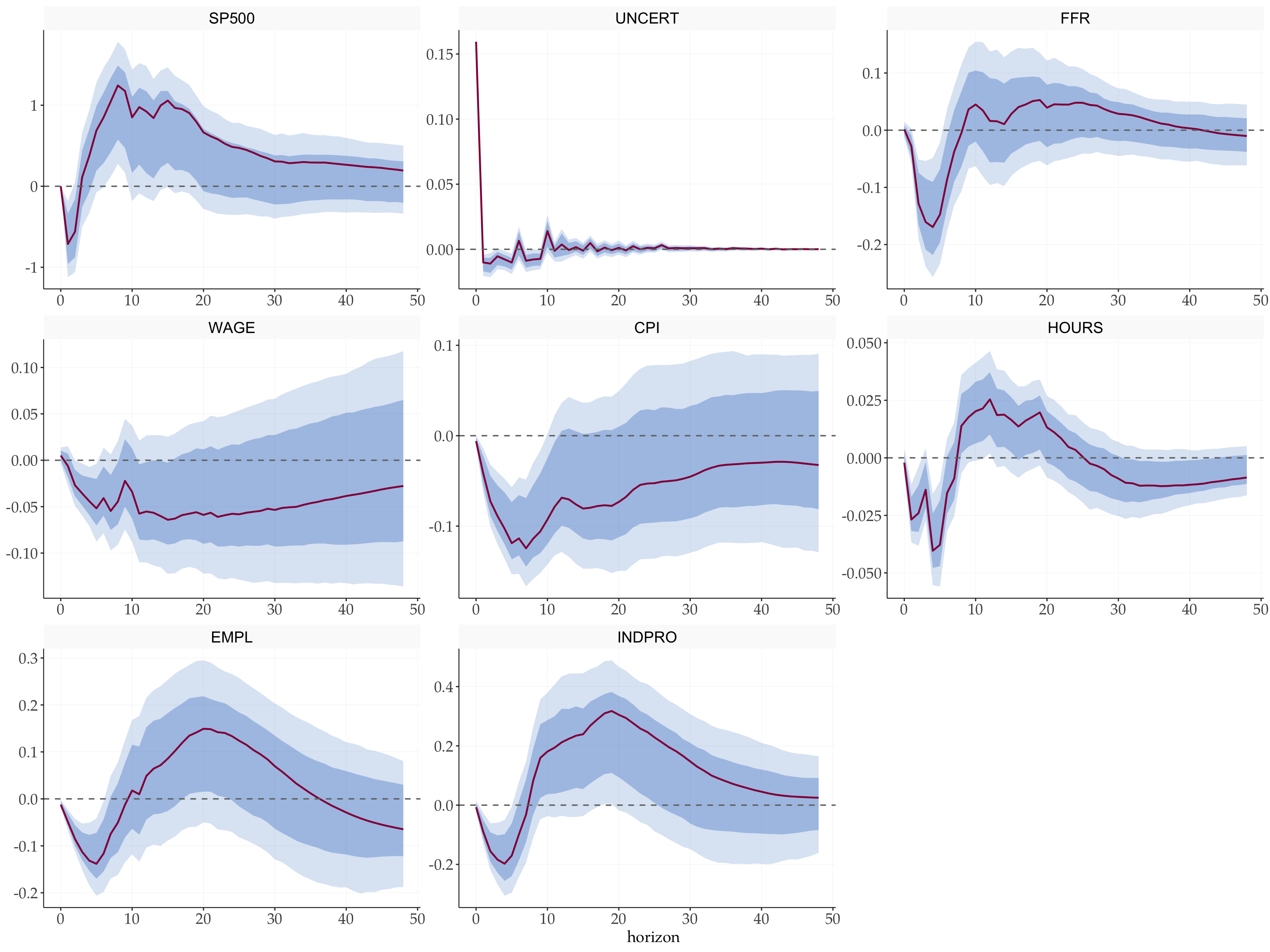

Figure 2.1: IRFs to uncertainty shock — standard bootstrap (68% and 90% confidence bands)

2.7.2 Bias-Corrected Bootstrap

fPlotIRFChol(
    point       = point_irf,
    boot_result = bloom_corrected,
    shock       = shock,
    varnames    = var_names,
    facet_ncol  = 3
) + 
    labs(y = NULL)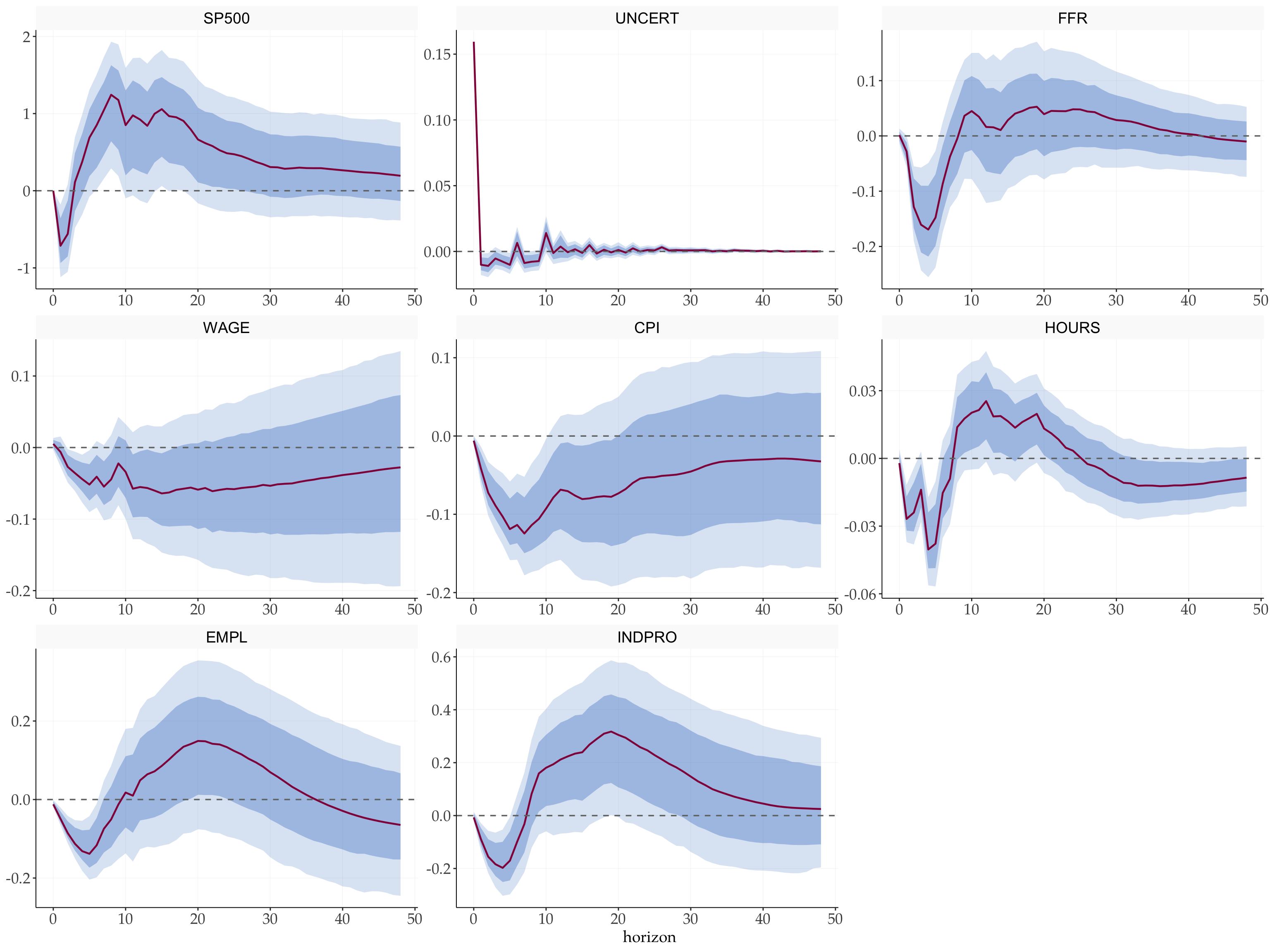

Figure 2.2: IRFs to uncertainty shock — bias-corrected bootstrap (68% and 90% confidence bands)

---

2.8 Forecast Error Variance Decomposition

Share of the \(h\)-step forecast error variance of variable \(k\) due to shock \(j\):

\[\mathrm{FEVD}_{k,j}(h) = \frac{\sum_{s=0}^{h-1} (\Theta_s)_{kj}^2}{\sum_{s=0}^{h-1} \sum_{\ell=1}^{K} (\Theta_s)_{k\ell}^2}.\]

vardec <- fFEVDChol(point_irf, shock = shock)

fPlotVarDec(
    fevd       = vardec$fevd,
    varnames   = var_names,
    shocknames = shockname
) +
  scale_fill_manual(values = tidyMacro_colors[c(2, 3)])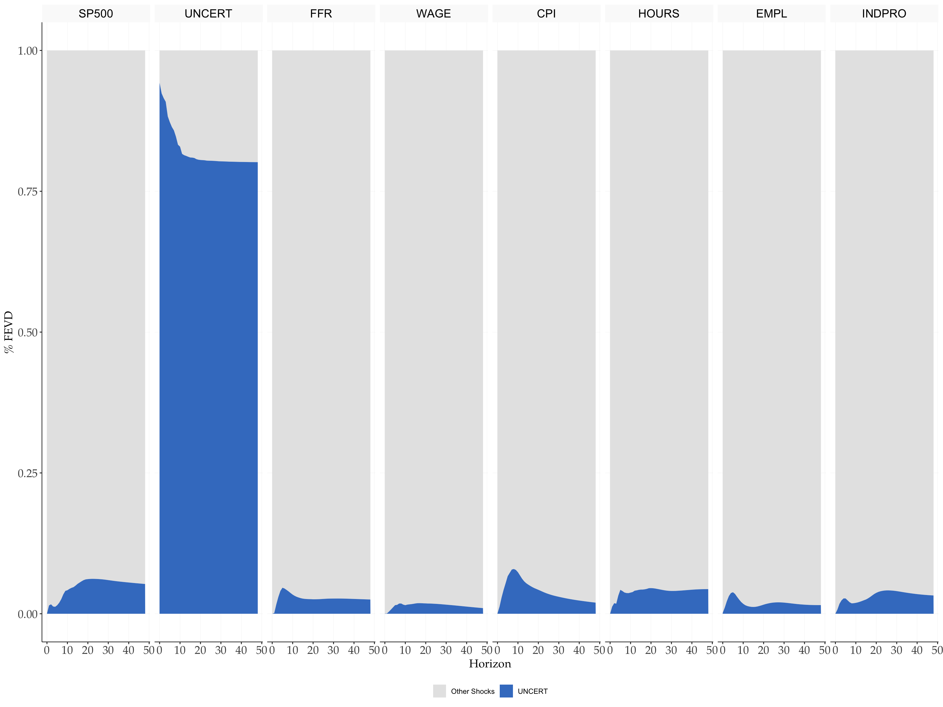

Figure 2.3: Forecast error variance decomposition: share explained by uncertainty shock

---

2.9 Historical Decomposition

Each observation decomposes into deterministic components plus cumulated shock contributions (companion form for \(p > 1\)):

\[y_t = \sum_{s=0}^{t-1} \Phi^s c + \Phi^t y_0 + \sum_{s=0}^{t-1} \Theta_s \varepsilon_{t-s}, \qquad HD_{k,t}^{(j)} = \sum_{s=0}^{t-1} (\Theta_s)_{kj}\, \varepsilon_{j,t-s}.\]

# Exclude the shock variable itself from the response variables
series <- setdiff(seq_len(N), shock)

histdec_list <- setNames(
    lapply(series, function(i) fHistDec(y, var_bloom, S, i)$histdec),
    colnames(y)[series]
)

fPlotHistDec(
    histdec_list = histdec_list,
    shock        = shock,
    shockname    = shockname,
    dates        = dates_vec,
    p            = p,
    facet_ncol   = 2
) +
    scale_x_date(date_breaks = "7 years", date_labels = "%Y")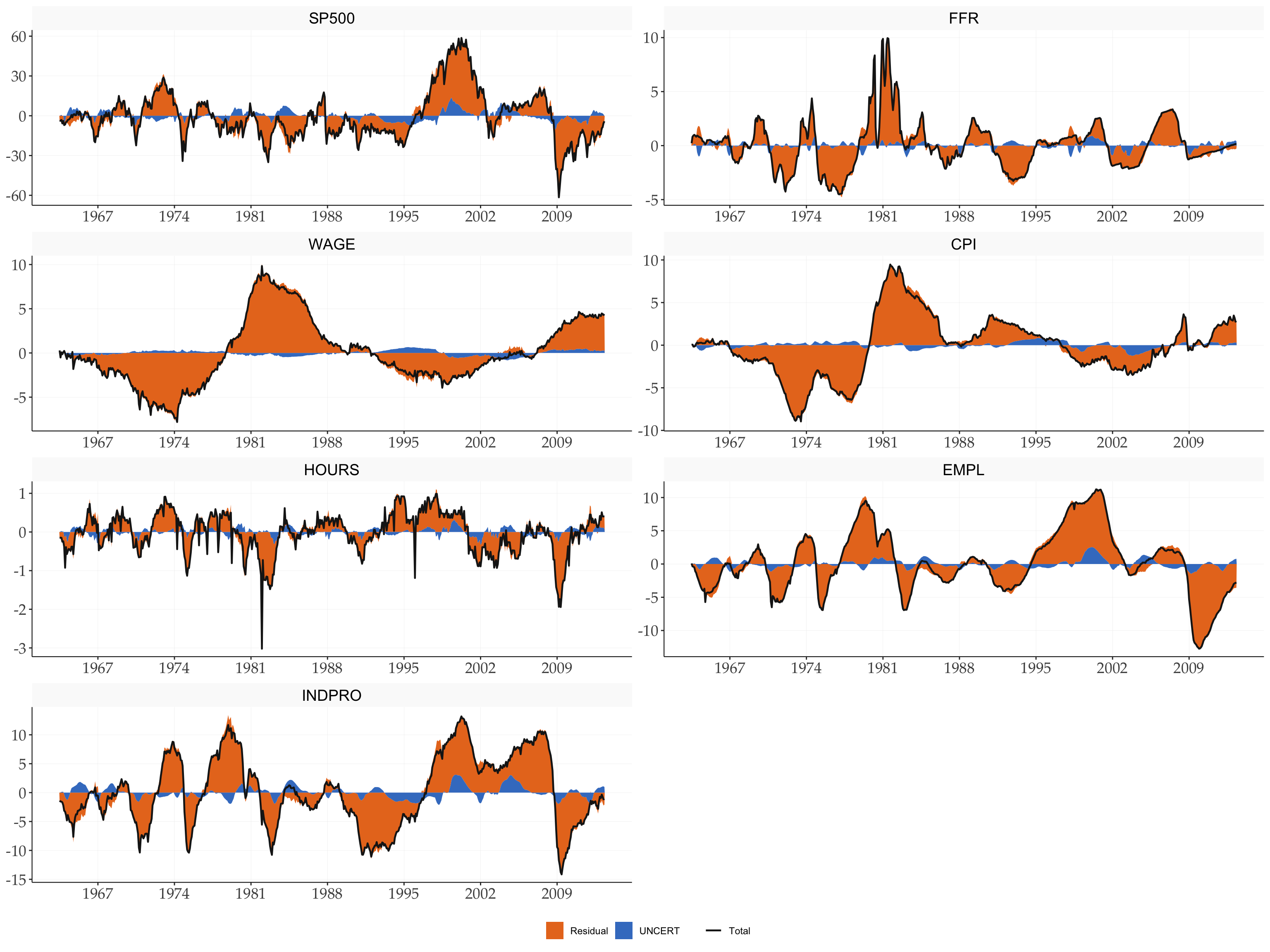

Figure 2.4: Historical decomposition: contribution of uncertainty shock

References

Bloom, Nicholas. 2009. “The Impact of Uncertainty Shocks.” Econometrica 77 (3): 623–85. https://doi.org/10.3982/ECTA6248.